Basics of VAEs and Diffusion Models

The dominant family of generative models today is the denoising diffusion probability models (DDPMs) due to its great capability of generating high-quality, fidelity-preserved images/videos. It's a generalization of variational auto-encoders (VAEs) that extends from one-step generation to multiple steps, mapping from a random probability space (usually Gaussian) to the data distribution space in a denoising manner. This blog post introduces the basics of VAEs and DDPMs and provides a simple application of generative models.

Preliminary: Variational Auto-Encoders (VAEs)

What do we want for generative models?

The ultimate goal of generative models is to model the real data distribution where is a data sample from the complete set of real data. However, it's usually infeasible for us access the full real dataset , so practically we use an observed dataset to approximate the real dataset and thus our goal is to model ths observed data distributiono where . Note that and are two different probability distributions.

Unfortunately, it's still impractical to model the observed data distribution for most of the time especially when the data samples are in a high dimensional space, like images, 3D objects and videos.

The generative models are purposed for modeling the observed data distribution from a given observed dataset , that is, estimating a new data distribution that approximates . After that, we can draw data samples from to generate new data samples.

Introduction to Auto-Encoders

Before we dive deep into VAEs, we first introduce what auto-encoders (AEs) are. AEs are a kind of models that first encode the given input into a high-dimensional representation , and then decode (which is called the latent variable) into . In this way, AEs are expected to learn the most import features embedded in . In other words, AEs implicitly learn the most significant features from the observed data distribution, through which we can expect to sample a new data sample by sampling a latent in the latent space.

However, as you may already notice, the problem is, how can we sample latents from the latent space. We know nothing about what the latent space is like: does is follow a normal distribution, a beta distribution, or a uniform distribution? We don't know! Sampling becomes a problem!

Another problem with AEs is, it's hard to measure the quality of the latent space. Presumably, if two data samples are similar, the encoded latent variables should also be similar, so that they can be further decoded back to the input. But this is not simply guaranteed!

To put the auto-encoding process more formally, we denote the parameterized encoder and decoder respectively as and . The auto-encoding process can be formulated as:

To train the auto-encoder, an loss is generally applied to enforce close to the ground-truth value :

For simple forms of and , we can sometimes get a closed form solution, but or neural networks, gradient descent is usually applied to solve and .

There are many variants of AEs to help learn a better latent space, and some works even quantize the latent space to get a finite set of latent variables. We will introduce these variants in future posts.

Understanding Variational Auto-Encoders

What is the distribution of the latent space?

As mentioned in the previous section, the biggest problem with AEs is that we cannot sample a latent in the latent space because we have no ideas what its distribution is. What if we can constrain, or enforce the latent distribution to be a simple well-known distribution, such as Gaussian distribution? Since we know the distribution, we can draw samples from this distribution and use the decode to generate the data sample.

Here come to us two remaining questions: - How can we constrain the latent distribution to be, like a Gaussian distribution? - How can we map our input data sample to this distribution, and teach the decoder to generate new data samples from this distribution?

Remember how we teach our AEs to learn decoding from to ? One simply idea is: we can add some loss to enforce the latants to approach a known distribution, e.g., a Gaussian distribution. With this loss, we can rewrite our training objective as:

The second loss, which we call reconstruction loss is unchanged as we want our AEs to learn to reconstruct the input sample. The new loss should teach our AEs to encode the input sample to a latent of a known distribution. How can we measure the closeness of two distributions? A natural measure would be the KL Divergence, which is defined as follows:

If both and are Gaussians, their KL divergeence has the following closed form (recall that the probability density of a random variable drawn from Gaussian is ):

To eliminate the second term, we notice that:

To eliminate the third term, we have:

Combining all three terms, we have:

When , the KL divergence can be simplified as:

It's a very nice simple closed form if we want to minimize the distance between the distribution of a standard Gaussian distribution! But wait, we still do not know the distribution of . What we all have are just these latents ! Wait a minute... instead of producing latents directly from the encoder, we can produce the mean and the variance matrix . If the elements of are independent with each other, we can further simplify to , i.e., . Once we have and , we can sample any latent by setting:

This is the so-called reparameterization trick, a technique that allows for efficient computation of gradients by sampling variables from a known distribution. More importanty in our case, it opens up the door for us to illuminate an explicit Gaussian distribution rather than an unknonwn distribution implicitly defined by the auto-encoder. This allows us to compute the KL divergence in a very simple way.

Combining all together, we have our final loss:

Theoretical derivation of VAEs

You may ask why this can or cannot work? Is the training objective really effective to push the latent distribution to a Gaussian and can we really sample a latent and generate a faithful new data point? So, we need to understand why this works under the hood, through a theorectical perspective.

Recall that our ultimate goal is to estimate the real data probability , but this is infeasible in practice. So in turn we can leverage a model parameterized by to estimate this probability, i.e., , and then our goal is to maximize the surrogate density.

In fact, the log probability can be rewritten as:

where can be any distribution parameterized by . The first term is the so-called evidence lower bound (ELBO) and the second term is the KL divergence between two distributions. If we can maximize ELBO, we can equivalently maximize the data log data distribution.

We can slightly rewrite the first term:

is the prior of latent variables. What do you find about the correlation of this formula to our empirical loss? Yes! They are equivalent if we take the negative of ELBO: one term minimizing the reconstruction loss and the other term minimizing the KL divergence.

The parameter is the encoder and is the decoder. What about the prior ? It can be anythingy, but a common choice would be a standard Gaussian distribution.

VAEs for Anime Face Generation

To demonstrate how VAEs work, let's use VAEs to generate anime faces, with data provided in this repository. You can use this piece of code. Don't forget to install the required packages.

However, training VAEs is not a trivial thing. As shown in the following figures, the generated images are quite blurry, missing details and lacking diversity.

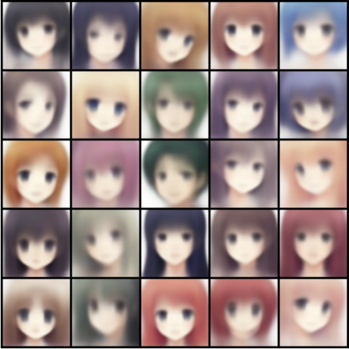
You can try yourself with the provided code, tune the loss weight for KL divergence. This may add some diversity but still, the generated images suffer from intensive blurs.

Understanding Denoising Diffusion Probability Models (DDPMs)

What is DDPMs

It seems quite simple for VAEs to learn to generate new data samples from a known distribution like Gaussians, but that's not trivial in fact. Imagine you have a high-dimensional dataset like real-world images that are characterized with bunches of features, and in this case, it's hard to model a perfect mapping from a standard Gaussian distribution to the real data distribution because the latter is very complex and the model is challenged to reconstruct the distribution space.

Diffusion models take a clever idea: generating a data sample from a single latent is hard, why not do it in multiple steps? That is, we first sample from a Gaussian distribution, and then decode it into a distribution that is close to Gaussian, and then decode this latent again, until the final decoded variable matches the real data distribution. Samping from a sequence of steps is much simpler compared to directly sampling from the Gaussian and decoding it into a real data sample in one step. To put it more simply, our latent is not a single variable any more, but a sequence of latents where is the number of diffusion steps. Instead of encoding an implicit , a sequence of Gaussian noises are progressively added to the original data point so that the more steps, the closer the latent variable approaches a true Gaussian. This is called the forward diffusion process.

Forward diffusion process

Given a data point , we can add a Gaussian noise to it in each of the steps, producing a sequence of noisy samples . We would like the probability distribution of given to be a Gaussian, which can be explicitly expressed as:

Here is a variance schedule controlling how much noise should be injected to the previous sample. Note that we use the reparameterization trick to sample from given . Then we can recursively express in terms of :

From the above equation, we have the full forward diffusion process: starting with a clean input and a specified timestep , we can produce a noised input by injecting a weighted standard Gaussian noise with predefined noise strength . Intuitive, a larger timestep results in a more noisy data point, so the sequence of noise strengths should meet .

We can represent in terms of :

Backward denoising process

What we're really interested in is the reverse process: how to get from . To this end, we must estimate , the backward denoising probability. However, this is intractable as we do not know neither nor . Fortunately, it's tractable to estimate :

Now is irrelevant to and has dependency on the timestep (or more specifically the noise ). We can thus rewrite the mean as .

What is the loss function? Recall that in the VAE section, we have derived the following lower bound:

If we regard as and as , we will have:

We can then decompose the lower bound into:

Maximizing the ELBO is equivalent maximing the reconstruction loss and minimizing KL divergences. Among the losses, we are interested in the KL divergence where is known given and and can be parameterized by neural networks.

Recall that the KL divergence bwtween two Gaussians and is:

In our case, is known, but is unknown. Similar to , we can simplify and parameterize as . Therefore, the final KL divergence can be:

The "ground-truth" mean as derived above is . As is known at training time, we can ask the model to predict only the noise for , which can be formulated as . Plug all these into the KL divergence and ignore variances:

Discarding the coefficient, we have the final loss function for time step :

That is, during training we randomly sample a time step and a Guassian noise , obtain , and predict the noise to the ground-truth .

As for , it's found that empirically set it to be or simply performs well enough. Learning a diagonal results in unstable training.

Choice of

The remaining question is how to choose the scheduler , or , or .

Recall that the noise is injected through and . The simplest scheduler is a linear function of , i.e.,:

with and . An improved scheduler is the cosine schduler:

This scheduler has an effect of a linear drop-off in the middle of the process and a more flat change near the extremes of and .

Classifier Guided Diffusion and Classifier-Free Guidance (CFG)

Classifier guided diffusion

In real-world applications, we usually want to control generation conditioning on some inputs, denoted by . Before introducing how to guide the diffusion models, let's visit one important formula:

by incorporating the reparameterization trick . In this way, we're connecting the derivative of the log-likelihood and the noise. Intuitively, the back-propagation update direction should be the inverse of the noise injected to the raw data point.

Now we'd like to estimate the derivative of the joint probability of :

Thus, becomes the new noise to approximate for time step . Here is an off-the-shelf classifier or classifier trained from scratch. We can also also a weight to the classifier part:

Classifier-free guidance

It's cumbersome to leverage an extra classifier to guide the diffusion process. Fortunately, by slightly re-write the score function, we can bypass the need of an additional classifier model:

is the predictor with guidance as input and is the predictor without guidance as input. In this formulation, there is not any explicit classifier. All we need is a unified diffusion model.

Diffusion Models for Anime Face Generation

Now, let's train diffusion models on the same anime face dataset. We use a simple U-Net as the model backbone and leverage the diffusers library to schedule noise. You can download the code here.

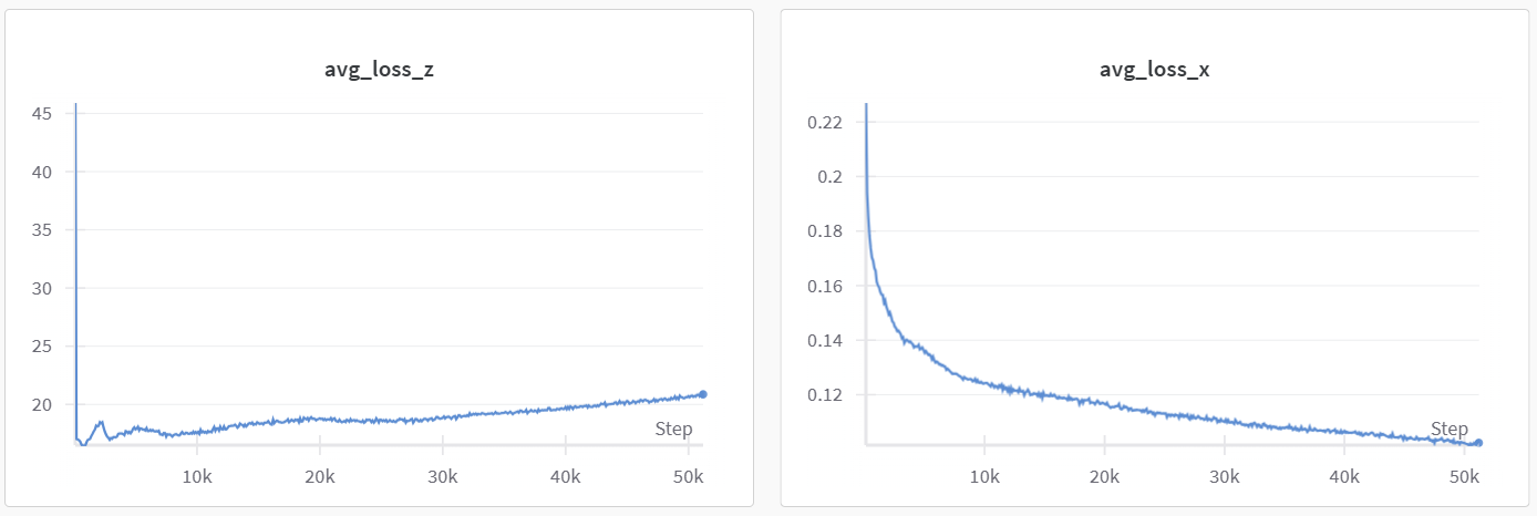
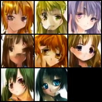
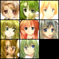
Training diffusion models takes much longer than VAEs before obtaining satisfactory results. You'll observe loss convergence soon after training but it does not mean the generated images are good enough. Instead, As training proceeds, the results are getting better. Here are some results after training for two epochs on my laptop. If you will, you can train the model longer for higher-quality images.

Conclusion

In this post, we revisited the basic concepts and principles of auto-encoders, variational auto-encoders and diffusion models, and how they evolved through time. Diffusion models are not designed to replace auto-encoders or VAEs, instead, they can be used in conjunction, such as the latent diffusion models (LDMs) for a trade-off between compression and performance. More specifically, VAEs are good at preserving high-level compositions whereas diffusion models capture more fine-grained details. It's possible to combine the best of both worlds through LDMs. There are some applications of diffusion models on computer games such as scene generation, 3D model generation, UV generation, etc. There is huge potential for such models to sparkle in the near future.