GAMES101疑难点及作业详解

很早之前就想跟着做完GAMES101，但是拖延症一直让我拖到了现在，我决定不再鸽下去！本篇Blog主要记录在GAMES101学习中遇到的疑难问题，整理Bonus Material，以及详解每一课的作业（含提高题）。如有任何错误、遗漏，欢迎读者指出赐教！

作业一

main.cpp

本次作业只需要实现main.cpp中的几个函数：get_view_matrix，get_model_matrix和get_projection_matrix，只需要按照课上讲的内容实现就行了，基本没有难度。下面是代码：

Eigen::Matrix4f get_view_matrix(Eigen::Vector3f eye_pos)
{
    Eigen::Matrix4f view = Eigen::Matrix4f::Identity();
    Eigen::Matrix4f translate;

    translate << 1, 0, 0, -eye_pos[0], 
                 0, 1, 0, -eye_pos[1], 
                 0, 0, 1, -eye_pos[2], 
                 0, 0, 0, 1;

    view = translate * view;
    return view;
}

Eigen::Matrix4f get_model_matrix(float rotation_angle)
{
    Eigen::Matrix4f model = Eigen::Matrix4f::Identity();

    model << std::cos(rotation_angle / 180.0f * MY_PI), -std::sin(rotation_angle / 180.0f * MY_PI), 0, 0,
             std::sin(rotation_angle / 180.0f * MY_PI), std::cos(rotation_angle / 180.0f * MY_PI),  0, 0,
             0, 0, 1, 0,
             0, 0, 0, 1;

    return model;
}

Eigen::Matrix4f get_projection_matrix(float eye_fov, float aspect_ratio,
                                      float zNear, float zFar) 
{
    Eigen::Matrix4f projection = Eigen::Matrix4f::Identity();
    Eigen::Matrix4f perspective = Eigen::Matrix4f::Identity();
    Eigen::Matrix4f orthogonal = Eigen::Matrix4f::Identity();

    float t = std::tan(eye_fov / 180.0f * MY_PI / 2.0f) * std::abs(zNear);
    float r = aspect_ratio * t;

    perspective << zNear, 0, 0, 0,
                   0, zNear, 0, 0,
                   0, 0, zNear + zFar, -zNear * zFar,
                   0, 0, 1, 0;
    
    orthogonal <<  1.0 / r, 0, 0, 0,
                   0, 1.0 / t, 0, 0,
                   0, 0, 2.0 / (zNear - zFar), 0,
                   0, 0, 0, 1;

    projection = orthogonal * perspective;

    return projection;

}

提高题：绕任意轴旋转

本次作业的提高题是实现向量绕任意轴旋转的旋转矩阵，推导过程见这篇博文。下面的代码是文章中描述的矩阵形式：

Eigen::Matrix4f get_rotation(Vector3f axis, float angle)
{
    float rotationRad = angle / 180.0f * MY_PI;

    Eigen::Matrix3f N = Eigen::Matrix3f::Identity();

    N << 0, -axis(2), axis(1),
         axis(2), 0, -axis(0),
         -axis(1), axis(0), 0;

    Eigen::Matrix3f R = Eigen::Matrix3f::Identity() + std::sin(rotationRad) * N + (1 - std::cos(rotationRad)) * N * N;

    Eigen::Matrix4f rotation = Eigen::Matrix4f::Identity();

    rotation.block(0, 0, 3, 3) = R;

    return rotation; 
}

作业二

本次作业的要求是实现光栅化与MSAA。作业需要完成：

• 为每个三角形创建2D Bounding Box；
• 判断点是否在三角形内；
• 判断深度值并更新深度缓存、颜色缓存；
• 使用MSAA抗锯齿。

insideTriangle函数

首先是判断点(x,y)是否在三角形内：

static bool insideTriangle(float x, float y, const Vector3f* _v)
{   
    // check if the point (x, y) is inside the triangle represented by _v[0], _v[1], _v[2]
    Vector3f pointA = _v[0];
    Vector3f pointB = _v[1];
    Vector3f pointC = _v[2];
    Vector3f pointO(x, y, 0.0f);
    
    Vector3f OA = pointA - pointO;
    Vector3f OB = pointB - pointO;
    Vector3f OC = pointC - pointO;

    float signOAB = OA.x() * OB.y() - OA.y() * OB.x();
    float signOBC = OB.x() * OC.y() - OB.y() * OC.x();
    float signOCA = OC.x() * OA.y() - OC.y() * OA.x();

    return signOAB >=0 && signOBC >=0 && signOCA >=0 || signOAB <=0 && signOBC <=0 && signOCA <=0;
}

这里使用的方法就是分别考察,和的值是否相同。因为我们只需要考察值，所以不用真的去计算叉乘，只需要根据公式算出值，然后比较是否相同即可。

rasterize_triangle函数

下面是rasterize_triangle函数代码：

void rst::rasterizer::rasterize_triangle(const Triangle& t) {
    auto v = t.toVector4();
    
    // Find out the bounding box of current triangle.
    // iterate through the pixel and find if the current pixel is inside the triangle
    int x_min = 1 << 5, x_max = -(1 << 5), y_min = 1 << 5, y_max = -(1 << 5);
    for (int i = 0; i < 3; ++i)
    {
        if (t.v[i].x() < x_min) x_min = t.v[i].x();
        if (t.v[i].x() > x_max) x_max = t.v[i].x();
        if (t.v[i].y() < y_min) y_min = t.v[i].y();
        if (t.v[i].y() > y_max) y_max = t.v[i].y();
    }

    for (float x = x_min; x <= x_max; ++x)
        for (float y = y_min; y <= y_max; ++y)
        {
            if (insideTriangle(x + 0.5, y + 0.5, t.v))
            {
                // If so, use the following code to get the interpolated z value.
                float z_interpolated = compute_interpolated_depth(x + 0.5, y + 0.5, t);
                if (z_interpolated < depth_buf[get_index(x, y)])
                {
                    depth_buf[get_index(x, y)] = z_interpolated;
                    set_pixel(Vector3f(x, y, 1.0f), t.getColor());
                }
            }
        }
}

这里为了代码简洁性，把计算深度插值单独提出去当一个函数：

float rst::rasterizer::compute_interpolated_depth(float x, float y, const Triangle& t)
{
    auto coefficients = computeBarycentric2D(x, y, t.v);

    float alpha, beta, gamma;
    std::tie(alpha, beta, gamma) = coefficients;

    return 1.0/(alpha / t.v[0].z() + beta / t.v[1].z() + gamma / t.v[2].z());
}

注意，原来代码框架提供的深度插值有误，正确的应是上面的版本（因为之前已经对w进行了归一化，使用原来版本的插值得到的是屏幕空间中的插值而非真实的深度插值）。推导过程详见矫正透视投影插值及属性插值详解。

提高题：实现MSAA

MSAA是把每个像素再拆分成几个小像素，每个小像素单独维护各自的深度和颜色，最后在计算大像素颜色的时候，只需要平均一下其内部小像素的颜色即可，深度则采取具有最小深度值小像素的深度：

void rst::rasterizer::rasterize_triangle(const Triangle& t) {
    auto v = t.toVector4();

    const float dx[4] = {0.25, 0.25, 0.75, 0.75}, dy[4] = {0.25, 0.75, 0.25, 0.75};
    
    // Find out the bounding box of current triangle.
    // iterate through the pixel and find if the current pixel is inside the triangle
    int x_min = 1 << 5, x_max = -(1 << 5), y_min = 1 << 5, y_max = -(1 << 5);
    for (int i = 0; i < 3; ++i)
    {
        if (t.v[i].x() < x_min) x_min = t.v[i].x();
        if (t.v[i].x() > x_max) x_max = t.v[i].x();
        if (t.v[i].y() < y_min) y_min = t.v[i].y();
        if (t.v[i].y() > y_max) y_max = t.v[i].y();
    }

    for (float x = x_min; x <= x_max; ++x)
        for (float y = y_min; y <= y_max; ++y)
        {
            int index = get_index(x, y) * 4;
            bool need_recompute_color = false;
            float pixel_depth = std::numeric_limits<float>::infinity();

            for (int i = 0; i < 4; ++i)
            {
                if (insideTriangle(x + dx[i], y + dy[i], t.v))
                {
                    // If so, use the following code to get the interpolated z value.
                    float z_interpolated = compute_interpolated_depth(x + dx[i], y + dy[i], t);
                    if (z_interpolated < depth_sample[index + i])
                    {
                        depth_sample[index + i] = z_interpolated;
                        frame_sample[index + i] = t.getColor();
                        // need_recompute_color is set to true if one sample depth updates
                        need_recompute_color = true; 
                        pixel_depth = std::min(pixel_depth, z_interpolated);
                    }
                }
            }

            if (need_recompute_color)
            {
                Vector3f color = (frame_sample[index] + frame_sample[index + 1] + frame_sample[index + 2] + frame_sample[index + 3]) / 4.0f;
                depth_buf[get_index(x, y)] = std::min(pixel_depth, depth_buf[get_index(x, y)]); // in fact, depth_buf is now useless when using MSAA
                set_pixel(Vector3f(x, y, 1.0f), color);
            }      
        } 
}

采用MSAA时要注意的是，并不是当前大像素的深度没有更新，其颜色就不用更新。这是因为大像素的颜色是由其内部的小像素的颜色平均而来，只要其中一个小像素的颜色改变了，大像素的颜色就要重新计算。而小像素颜色的变化是由小像素深度的变化引起的，所以，在考虑当前大像素时，只要其中任意一个小像素的深度更新了，那么就需要重新计算大像素的颜色。

布尔值need_recompute_color就用来记录当前大像素是否需要重新计算颜色，它只有在insideTriangle(x + dx[i], y + dy[i], t.v)为True（即当前小像素在三角形内），和z_interpolated < depth_sample[index + i]时（即小像素的深度值得到更新）才为True。

代码

if (need_recompute_color)
{
    Vector3f color = (frame_sample[index] + frame_sample[index + 1] + frame_sample[index + 2] + frame_sample[index + 3]) / 4.0f;
    depth_buf[get_index(x, y)] = std::min(pixel_depth, depth_buf[get_index(x, y)]); // in fact, depth_buf is now useless when using MSAA
    set_pixel(Vector3f(x, y, 1.0f), color);
}

把当前大像素内所有小像素的颜色平均起来，就是最终呈现在屏幕上的颜色。

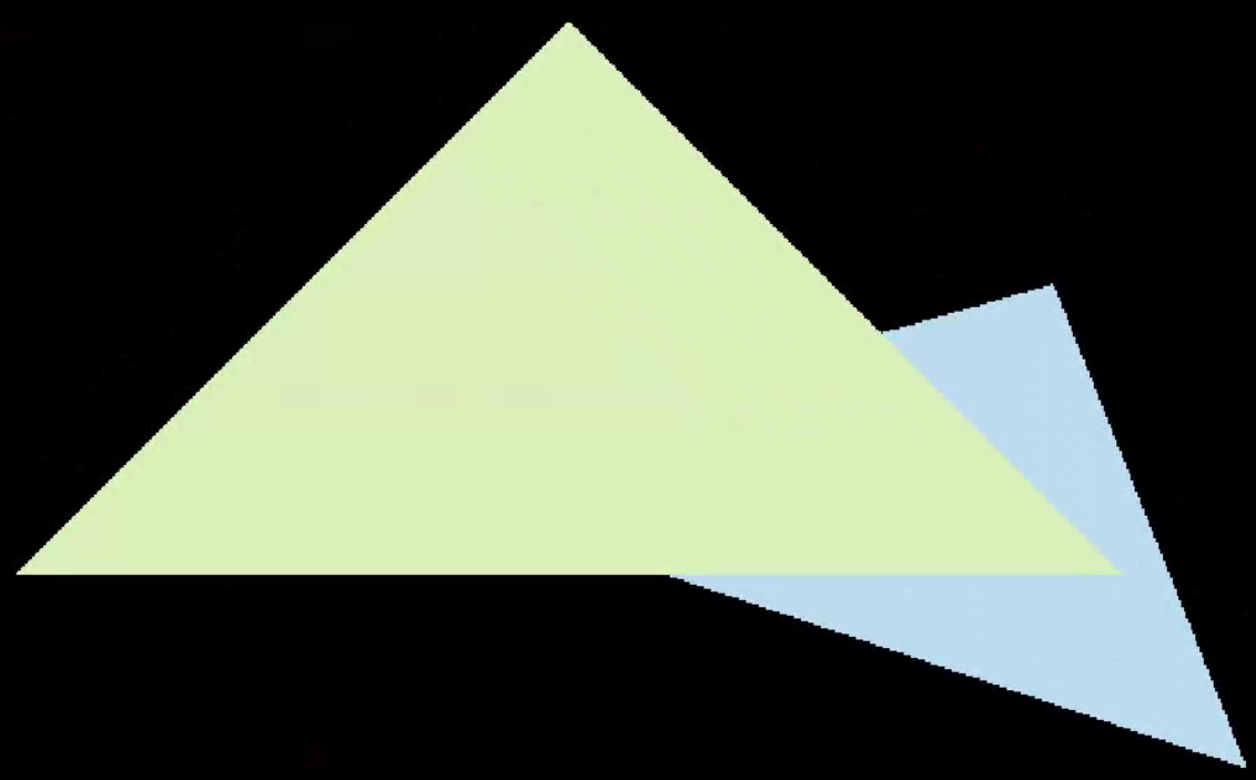
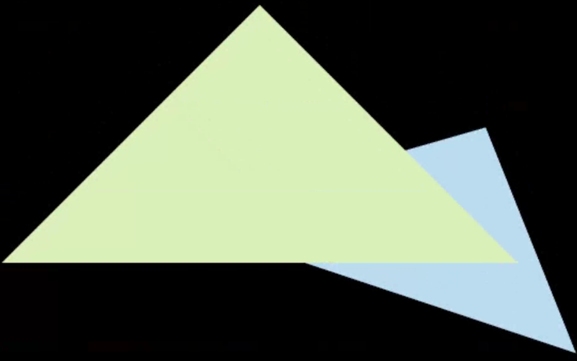
下面的两图对比了无MSAA和有MSAA的效果，可以看到没有MSAA时，蓝色三角形有明显锯齿，而加了MSAA之后，锯齿得到了显著改善。

作业三

本次作业要求实现：

• Normal、Color、Texture Interpolation;
• Blinn-Phong Reflection Model / Texture Mapping / Bump Mapping / Displacement Mapping;
• Bilinear Interpolation.

实际上只完成作业要求并不困难，更为重要的是要理解整套渲染的逻辑。因此，下面将按照渲染处理流程解析代码框架，在这个过程中完成作业。

The main function in main.cpp

Loading triangles from .obj file

整个程序从main.cpp的main函数开始执行，前几行读取了.obj模型文件，每个模型文件都包含了若干个三角形的每个顶点的位置坐标、法向量和纹理坐标。下面的代码把这些三角形存储为一个数组：

for(auto mesh:Loader.LoadedMeshes)
    {
        for(int i=0;i<mesh.Vertices.size();i+=3)
        {
            // Instantiate a new triangle
            Triangle* t = new Triangle();
            for(int j=0;j<3;j++)
            {
                // Store the position
                t->setVertex(j,Vector4f(mesh.Vertices[i+j].Position.X,mesh.Vertices[i+j].Position.Y,mesh.Vertices[i+j].Position.Z,1.0));
                // Store the normal
                t->setNormal(j,Vector3f(mesh.Vertices[i+j].Normal.X,mesh.Vertices[i+j].Normal.Y,mesh.Vertices[i+j].Normal.Z));
                // Store the texture coordinate
                t->setTexCoord(j,Vector2f(mesh.Vertices[i+j].TextureCoordinate.X, mesh.Vertices[i+j].TextureCoordinate.Y));
            }
            TriangleList.push_back(t);
        }
    }

如果你有兴趣，可以打开OBJ_Loader.h查看如何加载模型。

Building a rasterizer and setting up the shader

下一步就是构建一个光栅化器，然后设置想要的Shader：

// Instantiate the rasterizer
rst::rasterizer r(700, 700);

auto texture_path = "hmap.jpg";
r.set_texture(Texture(obj_path + texture_path));

// Set the default shader
std::function<Eigen::Vector3f(fragment_shader_payload)> active_shader = phong_fragment_shader;

if (argc >= 2)
{
    command_line = true;
    filename = std::string(argv[1]);

    // The following lines set different shaders according to the input parameter
    if (argc == 3 && std::string(argv[2]) == "texture")
    {
        std::cout << "Rasterizing using the texture shader\n";
        active_shader = texture_fragment_shader;
        texture_path = "spot_texture.png";
        r.set_texture(Texture(obj_path + texture_path));
    }
    else if (argc == 3 && std::string(argv[2]) == "normal")
    {
        std::cout << "Rasterizing using the normal shader\n";
        active_shader = normal_fragment_shader;
    }
    else if (argc == 3 && std::string(argv[2]) == "phong")
    {
        std::cout << "Rasterizing using the phong shader\n";
        active_shader = phong_fragment_shader;
    }
    else if (argc == 3 && std::string(argv[2]) == "bump")
    {
        std::cout << "Rasterizing using the bump shader\n";
        active_shader = bump_fragment_shader;
    }
    else if (argc == 3 && std::string(argv[2]) == "displacement")
    {
        std::cout << "Rasterizing using the bump shader\n";
        active_shader = displacement_fragment_shader;
    }
}

具体每个shader的实现在main.cpp中，在下文会详解。在这里只需要知道每个shader都是用不同的方法给每个像素着色即可。具体使用的shader存储在active_shader中，它接受一个类型为fragment_shader_payload的参数，存储的是当前像素点的一些信息（比如颜色、在view_space中的位置、法向量、纹理坐标等，view_space的含义下文解释），并返回一个Vector3类型的变量，代表当前像素要着色的RGB颜色。

可以把fragment_shader_payload理解为当前待着色的像素的信息，充当一个存储区，而不同的shader就根据自身的算法从fragment_shader_payload里调取需要的信息进行着色计算，返回最终的颜色。

Constructing MVP transformation and draw the image

main函数的最后几行就是构建MVP变换矩阵，然后调用光栅化器的draw函数：

r.clear(rst::Buffers::Color | rst::Buffers::Depth);
r.set_model(get_model_matrix(angle));
r.set_view(get_view_matrix(eye_pos));
r.set_projection(get_projection_matrix(45.0, 1, 0.1, 50));

r.draw(TriangleList);

The projection matrix

不要忘了把作业二中的projection matrix代码拷贝过来：

Eigen::Matrix4f get_projection_matrix(float eye_fov, float aspect_ratio, float zNear, float zFar)
{
    Eigen::Matrix4f projection;

    double d = 1 / tan((eye_fov/2) * MY_PI / 180); 
    double A = -(zFar + zNear) / (zFar - zNear); 
    double B = -2 * zFar * zNear / (zFar - zNear); 
    projection << d / aspect_ratio, 0, 0, 0, 
                    0, d, 0, 0, 
                    0, 0, A, B, 
                    0, 0, -1, 0;  

    return projection;
}

The draw function in rasterizer.cpp

在main函数中，我们已经准备好了每个三角形的信息、要用的着色器和MVP变换矩阵，下面就是要根据这些信息计算屏幕空间中每个像素的颜色。

Transform each vertex into the view space

由于上面的每个三角形中的顶点都是在世界坐标中，第一步要做的就是用MVP变换矩阵把它们转换到另外的空间中。

这里尤其需要注意的是，我们实际上有三个不同的空间，或者说坐标系：

• View space: 这是顶点经过MV变换后的坐标，点经过MV变换后的点（注意顺序）实际上位于相机的局部坐标系中（camera's local space），我们称之为view space。
• Projection space: 这是顶点经过完整的MVP变换后的坐标，也即，此时点的深度值会被透视投影改变，所以此时的深度并不代表点在真实三维空间中的深度，而是为了模拟人眼效果做出的变换，这也就是为什么我们要保留点在view space中的信息，因为在view space中的深度值才是点在真实世界中的值。
• Screen space: 这是点经过视口变换后得到的坐标，此时点的深度值不再重要，我们只关心它的，也即在屏幕上的位置。

值得注意的是，某原始三维空间（未经过任何变换）中的点，与它在view space/projection space/screen space中的点是能对应起来的，在计算的时候，要注意把它们当成一个整体考虑。比如原始三维空间中的点，其在view space/projection space/screen space中的点分别为，那么就要把联系起来考虑，不要孤立地看任何一个点。

回到代码中，下面的代码首先得到了整个MVP变换矩阵：

Eigen::Matrix4f mvp = projection * view * model;

而draw函数整体是一个大循环，对每个三角形进行计算：

for (const auto& t:TriangleList)
{
    Triangle newtri = *t;
    ...
}

下面的代码把每个顶点变换到view space中：

/*      Compute `viewspace_pos`, which represents the camera's local space coordinates without projection transformation  */
/*      This position will then be used for shading.                                                                      */
        std::array<Eigen::Vector4f, 3> mm {
                (view * model * t->v[0]),
                (view * model * t->v[1]),
                (view * model * t->v[2])
        };

        std::array<Eigen::Vector3f, 3> viewspace_pos;

        std::transform(mm.begin(), mm.end(), viewspace_pos.begin(), [](auto& v) {
            return v.template head<3>();
        });

此时viewspace_pos里存的就是三角形三个顶点在view space中的坐标。

Transform each vertex into the projection space

当然我们还需要把每个顶点转变到projection space中：

/*      Compute `v` with mvp transformation   */
        Eigen::Vector4f v[] = {
                mvp * t->v[0],
                mvp * t->v[1],
                mvp * t->v[2]
        };

此时，v里存的就是三角形三个顶点在projection space的坐标。更关键的是下面的几行代码:

/*      Now `vec.w()` records the original `z` value before applying projection transformation    */
/*      Note that it is different from the formulation in Assignment 2                            */
        for (auto& vec : v) {
            vec.x() /= vec.w();
            vec.y() /= vec.w();
            vec.z() /= vec.w();
        }

在这里，每个顶点都除以其向量的w分量，使其得到正确的坐标，而这里的w，正是view space中的z值，也就是经过MV变换后的深度值！此处没有对w分量归一化是因为后面插值时还需要用到view space中的z值，也就是点在真实空间中的深度值。

Transform the normal into the view space

既然顶点已经被变换到view space中了，那么每个顶点的法向量也需要变换到view space中，这可以用下面的代码描述：

/*      Transform the world space normal vectors into camera's local space coordinates.       */
/*      Need a little bit mathematics.                                                        */
        Eigen::Matrix4f inv_trans = (view * model).inverse().transpose();
        Eigen::Vector4f n[] = {
                inv_trans * to_vec4(t->normal[0], 0.0f),
                inv_trans * to_vec4(t->normal[1], 0.0f),
                inv_trans * to_vec4(t->normal[2], 0.0f)
        };

注意，法向量并不能简单像顶点那样直接进行MV变换，即乘以矩阵，而是乘了，推导如下：

假设变换前的法向量是，它的任意切线是，变换矩阵是，变换后的法线和切线分别是，其中，那么下面的式子成立：

令上面两式相等，则有：

由于是任意切向量，所以有：

所以对法向量来说，要把它变换到view space，需要乘的矩阵是。

Apply viewport projection and store infomation

最后只需要应用视口变换及存储上面计算的信息即可：

//Viewport transformation
for (auto & vert : v)
{
    vert.x() = 0.5*width*(vert.x()+1.0);
    vert.y() = 0.5*height*(vert.y()+1.0);
    vert.z() = vert.z() * f1 + f2;
}

for (int i = 0; i < 3; ++i)
{
    //screen space coordinates
    newtri.setVertex(i, v[i]);
}

for (int i = 0; i < 3; ++i)
{
    //view space normal
    newtri.setNormal(i, n[i].head<3>());
}

newtri.setColor(0, 148,121.0,92.0);
newtri.setColor(1, 148,121.0,92.0);
newtri.setColor(2, 148,121.0,92.0);

再回顾一下，newtri.seetVertex(i, v[i])存储的是screen space的坐标，每个顶点的分量则是view space的深度值，也就是点在真实空间中的深度值。newtri.setNormal(i, n[i].head<3>())存储的是点在view space中的法向量。

之后调用rasterize_triangle(newtri, viewspace_pos)给每个三角形光栅化和着色。注意这里既传入了newtri，也传入了viewspace_pos，这是因为我们需要顶点在真实空间中的坐标位置。

The rasterize_triangle function in rasterizer.cpp

函数rasterize_triangle是真正执行光栅化和着色的地方，主要需要实现每个像素的属性插值，并调用之前定义的shader去着色。

下面我仍然使用作业二的MSAA去实现，但是由于给的模型面数较少，所以使用MSAA与不使用MSAA区别不大，特此说明。

之后的所有代码都按照顺序实现在rasterize_triangle函数中：

void rst::rasterizer::rasterize_triangle(const Triangle& t, const std::array<Eigen::Vector3f, 3>& view_pos) 
{
    ...
}

Define variables and get the bounding box

第一步是先定义一些需要的变量，找到当前三角形在screen space中的bounding box：

// USed for MSAA
const float dx[4] = {0.25, 0.25, 0.75, 0.75}, dy[4] = {0.25, 0.75, 0.25, 0.75};

auto v = t.toVector4();

// Get the bounding box
int x_min = 1 << 5, x_max = -(1 << 5), y_min = 1 << 5, y_max = -(1 << 5);
for (int i = 0; i < 3; ++i)
{
    if (t.v[i].x() < x_min) x_min = t.v[i].x();
    if (t.v[i].x() > x_max) x_max = t.v[i].x();
    if (t.v[i].y() < y_min) y_min = t.v[i].y();
    if (t.v[i].y() > y_max) y_max = t.v[i].y();
}

Iterate each pixel and sub-pixel

第二步是对每个像素，对里面的每个子像素进行操作。首先需要定义整体的结构：

// Iterate each pixel
for (float x = x_min; x <= x_max; ++x)
    for (float y = y_min; y <= y_max; ++y)
    {
        // If set to `true`, the current pixel needs reshading
        bool need_reshading = false;
        float pixel_depth = std::numeric_limits<float>::infinity();
        
        int index = get_index(x, y) * 4;

        for (int i = 0; i < 4; ++i)
        {
            if (insideTriangle(x + dx[i], y + dy[i], t.v))
            {
                // Do something for each sub-pixel if it's inside the triangle
                ...
            }
        }

        if (need_reshading)
        {
            set_pixel(Vector2i(x, y), (frame_sample[index] + frame_sample[index + 1] + frame_sample[index + 2] + frame_sample[index + 3]) / 4);
            depth_buf[get_index(x, y)] = std::min (depth_buf[get_index(x, y)], pixel_depth);
        }
    }

在这里，我们首先考虑每个像素。每个像素定义了一个布尔值need_reshading，它表示如果像素内部有小像素的颜色发生变化，那么大像素就需要重新着色，那就是把内部几个小像素（这里用了四个）的颜色值进行平均，这就是代码set_pixel(Vector2i(x, y), ...);做的事情。而pixel_depth则更新大像素的深度值。

为了使用MSAA，我们仍然需要像作业二一样另开两个数组去分别记录每个子像素的颜色和深度，记为frame_sample和depth_sample。

接下来就是要对每个在三角形内的子像素进行操作了。

Calculate the interpolated depth

对每个在三角形内的子像素，首先需要计算它在screen space中的重心坐标，然后利用重心坐标去算深度插值：

// Calculate the interpolated depth value `z_interpolated`
auto coefficients = computeBarycentric2D(x + dx[i], y + dy[i], t.v);

float alpha, beta, gamma;
std::tie(alpha, beta, gamma) = coefficients;

// Doing interpolation in the camera's local space, i.e., before projection transformation
// The resulting `z_interpolated` is the interpolated depth after projection transformation
float Z = 1.0 / (alpha / t.v[0].w() + beta / t.v[1].w() + gamma / t.v[2].w());
float zp = alpha * t.v[0].z() / t.v[0].w() + beta * t.v[1].z() / t.v[1].w() + gamma * t.v[2].z() / t.v[2].w();
float z_interpolated = zp * Z;

computeBarycentric2D是给定的代码不用处理，得到的alpha，beta和gamma就是三个顶点对应的重心坐标值。

后面三行代码需要注意！之前我们提到，三角形三个顶点向量的w分量实际上是三角形在view space，也就是在真实空间中的深度值，那么在进行插值的时候，就需要用这个真实的深度值去计算得到当前像素点在view space中的深度值，也就是这里的变量Z。

但是我们人眼看到的，实际上是在projection space中的深度，也就是经过MVP变换后的深度，所以此时就可以把projection space中的深度视为一种“属性”，应用这篇博客中介绍的原理，插值得到当前像素点在projection space中的深度，也就是z_interpolated。

实际上这个插值算法可以用于任何属性的插值而不仅仅是projection space中的深度值，而原本的代码中的两个interpolate函数只是在屏幕空间中插值，是错误的，所以下面我首先对这两个interpolate函数进行修改：

static Eigen::Vector3f interpolate(const Triangle& t, float alpha, float beta, float gamma, const Eigen::Vector3f& vert1, const Eigen::Vector3f& vert2, const Eigen::Vector3f& vert3, float weight)
{
/*
    return (alpha * vert1 + beta * vert2 + gamma * vert3) / weight;
*/
    float Z = 1.0 / (alpha / t.v[0].w() + beta / t.v[1].w() + gamma / t.v[2].w());
    Vector3f interpolated = alpha * vert1 / t.v[0].w() + beta * vert2 / t.v[1].w() + gamma * vert3 / t.v[2].w();
    Vector3f interpolated_attribute = interpolated * Z / weight;
    return interpolated_attribute;
}

static Eigen::Vector2f interpolate(const Triangle& t, float alpha, float beta, float gamma, const Eigen::Vector2f& vert1, const Eigen::Vector2f& vert2, const Eigen::Vector2f& vert3, float weight)
{
/*
    auto u = (alpha * vert1[0] + beta * vert2[0] + gamma * vert3[0]);
    auto v = (alpha * vert1[1] + beta * vert2[1] + gamma * vert3[1]);

    u /= weight;
    v /= weight;

    return Eigen::Vector2f(u, v);
*/
    float Z = 1.0 / (alpha / t.v[0].w() + beta / t.v[1].w() + gamma / t.v[2].w());
    Vector2f interpolated = alpha * vert1 / t.v[0].w() + beta * vert2 / t.v[1].w() + gamma * vert3 / t.v[2].w();
    Vector2f interpolated_attribute = interpolated * Z / weight;
    return interpolated_attribute;
}

作为对比，原来的代码被注释掉了。现在插值得到的值，才是在真实空间中的值。

Get other interpolated attributes

最后只需要调用interpolate函数得到其他属性的插值即可。但首先要注意先判断一下深度：

if (z_interpolated < depth_sample[index + i])
{
    // Update depth of the current sub-pixel
    depth_sample[index + i] = z_interpolated;
    // Set `need_reshading` to true
    need_reshading = true;
    pixel_depth = std::min(pixel_depth, z_interpolated);

    auto interpolated_color = interpolate(t, alpha, beta, gamma, t.color[0], t.color[1], t.color[2], 1);
    // `normal` is in the view space
    auto interpolated_normal = interpolate(t, alpha, beta, gamma, t.normal[0], t.normal[1], t.normal[2], 1); 
    auto interpolated_texcoords = interpolate(t, alpha, beta, gamma, t.tex_coords[0], t.tex_coords[1], t.tex_coords[2], 1);
    // `interpolated_shadingcoords` is in the view space
    auto interpolated_shadingcoords = interpolate(t, alpha, beta, gamma, view_pos[0], view_pos[1], view_pos[2], 1);

    // Store the color/normal/texcoords/texture information into `fragment_shader_payload`
    fragment_shader_payload payload (interpolated_color, interpolated_normal.normalized(), interpolated_texcoords, texture ? &*texture : nullptr);
    payload.view_pos = interpolated_shadingcoords;
    // Instead of passing the triangle's color directly to the frame buffer, pass the color to the shaders first to get the final color;
    auto pixel_color = fragment_shader(payload);


    // Store the sub-pixel's color
    frame_sample[index + i] = pixel_color;
}

首先更新了当前子像素的深度，并把need_reshading设为true。之后调用interpolate计算得到颜色值、法线值、纹理坐标和view space中的深度值，然后把这所有的信息都存到fragment_shader_payload中，最后再调用选择的着色器fragment_shader计算当前子像素的颜色并存到frame_sample中。

到此为止，rasterize_triangle函数中的内容已经介绍完毕。

Try calling the normal_fragment_shader

最后的问题就是我们调用的着色器fragment_shader究竟是怎样的。所有的shader都定义在main.cpp中，且原始代码已经给我们提供了现成的normal_fragment_shader了:

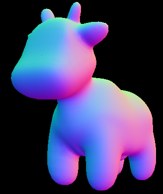
Eigen::Vector3f normal_fragment_shader(const fragment_shader_payload& payload)
{
    Eigen::Vector3f return_color = (payload.normal.head<3>().normalized() + Eigen::Vector3f(1.0f, 1.0f, 1.0f)) / 2.f;
    Eigen::Vector3f result;
    result << return_color.x() * 255, return_color.y() * 255, return_color.z() * 255;
    return result;
}

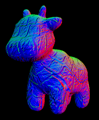
normal_fragment_shader做的实际上就是把像素对应的法向量归一化到区间，然后再乘以作为颜色值输出。

我们可以通过在终端输入./Rasterizer output.png normal查看结果，如下图所示：

我们可以把指令中的normal参数替换为其他参数：

• texture: 调用texture_fragment_shader，使用纹理坐标着色；
• phong: 调用phong_fragment_shader，使用blinn-Phong模型着色；
• bump：调用bump_fragment_shader，使用Bump Mapping着色；
• displacement：调用displacement_fragment_shader，使用Displacement Mapping着色。

下面，我们就依次实现这几个着色器。

Implement shaders

为了方便参考起见，先把blinn-Phong Reflection Model的计算公式放在此处：

blinn-Phong shader

phong_fragment_shader的整体代码如下：

Eigen::Vector3f phong_fragment_shader(const fragment_shader_payload& payload)
{
    // Ambient coefficient, diffuse coefficient and specular coefficient,
    // each is represented as an RBG color
    Eigen::Vector3f ka = Eigen::Vector3f(0.005, 0.005, 0.005);
    Eigen::Vector3f kd = payload.color;
    Eigen::Vector3f ks = Eigen::Vector3f(0.7937, 0.7937, 0.7937);

    // Light position and intensity in the view space
    auto l1 = light{{20, 20, 20}, {500, 500, 500}};
    auto l2 = light{{-20, 20, 0}, {500, 500, 500}};

    std::vector<light> lights = {l1, l2};
    Eigen::Vector3f amb_light_intensity{10, 10, 10};
    Eigen::Vector3f eye_pos{0, 0, 10};

    // Cosine power
    float p = 150;

    Eigen::Vector3f color = payload.color;
    Eigen::Vector3f point = payload.view_pos;
    Eigen::Vector3f normal = payload.normal;

    Eigen::Vector3f result_color = {0, 0, 0};
    for (auto& light : lights)
    {
        // Calculate the square distance r^2
        float square_distance = (light.position - point).squaredNorm();

        // Calculate the light direction, view direction, normal, and half vector
        Vector3f l = (light.position - point).normalized();
        Vector3f v = (eye_pos - point).normalized();
        Vector3f n = normal.normalized();
        Vector3f h = (l + v).normalized();
        
        // The light intensity
        Vector3f I = light.intensity;

        // Calculate the ambient light, diffuse light and specular light
        Vector3f ambient_light = ka.cwiseProduct(amb_light_intensity);
        Vector3f diffuse_light = kd.cwiseProduct(I / square_distance) * std::max(0.0f, n.dot(l));
        Vector3f specular_light = ks.cwiseProduct(I / square_distance) * std::pow(std::max(0.0f, n.dot(h)), p);

        result_color += ambient_light + diffuse_light + specular_light;
    }

    return result_color * 255.f;
}

首先定义了环境光、漫反射和镜面反射的三个颜色系数ka，kd和ks，每个系数都是一个RBG值。

然后，定义了两个光线，包括它们的位置和强度。注意强度也是一个三维向量，对颜色的三个分量各有一个强度值。

amb_light_intensity是环境光的强度，是一个与光线无关的定值；eye_pos是观测点；p用于镜面反射的余弦指数；color无用；point是当前像素在真实空间中的位置（着色点），normal是对应的法向量。

之后对每束光，依次计算光线到着色点的距离平方、光线方向、观测方向和半程向量，然后再用上述的公式计算得到环境光、漫反射光和镜面反射光即可。这里再说明下，光照强度Intensity可以理解为对颜色值的一种加权，强度越大，说明越突出当前颜色，或者说，该颜色被反射得越多；反之，则说明该颜色被吸收得越多。

此外，最后得到的result_color有可能某个分量的值大于1，理论上讲需要将其裁到的范围，但是后面用到的OpenCV可能会进行这个操作，所以这里就不进行裁剪了。

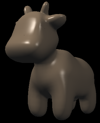
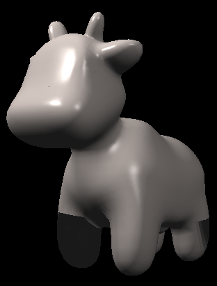
下图是blinn-Phong着色器得到的结果：

Texture shader

texture_fragment_shader的代码如下：

if (payload.texture)
{
    // The (u, v) texture coordinate of the current pixel
    Vector2f tex_coord = payload.tex_coords;
    // Get the color from texture
    return_color = payload.texture->getColor (tex_coord[0], tex_coord[1]);
}
Eigen::Vector3f texture_color;
texture_color << return_color.x(), return_color.y(), return_color.z();
...
Eigen::Vector3f kd = texture_color / 255.f;

和phong_fragment_shader唯一的不同在于这里的漫反射系数kd是通过纹理上的颜色设置的，其他计算过程都完全一致。

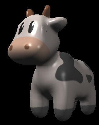
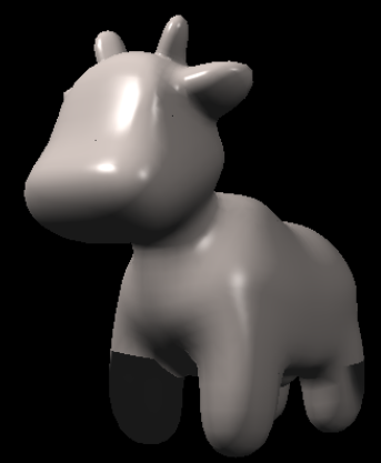
下图是texture_fragment_shader得到的结果：

Bump shader

Bump mapping之后会写一篇文章介绍，在这里直接搬运别人的代码如下（注: 已更新对凹凸贴图的详解）：

Eigen::Vector3f bump_fragment_shader(const fragment_shader_payload& payload)
{
    
    Eigen::Vector3f ka = Eigen::Vector3f(0.005, 0.005, 0.005);
    Eigen::Vector3f kd = payload.color;
    Eigen::Vector3f ks = Eigen::Vector3f(0.7937, 0.7937, 0.7937);

    auto l1 = light{{20, 20, 20}, {500, 500, 500}};
    auto l2 = light{{-20, 20, 0}, {500, 500, 500}};
e
    std::vector<light> lights = {l1, l2};
    Eigen::Vector3f amb_light_intensity{10, 10, 10};
    Eigen::Vector3f eye_pos{0, 0, 10};

    float p = 150;

    Eigen::Vector3f color = payload.color; 
    Eigen::Vector3f point = payload.view_pos;
    Eigen::Vector3f normal = payload.normal;

    //
    float kh = 0.2, kn = 0.1;

    //
    Vector3f n = normal.normalized();
    float d = sqrt(n.x() * n.x() + n.z() * n.z());
    Vector3f t (n.x() * n.y() / d, d, n.z() * n.y() / d);
    Vector3f b = n.cross(t);

    Matrix3f TBN;
    TBN.col(0) = t, TBN.col(1) = b, TBN.col(2) = n;

    float u = payload.tex_coords.x(), v = payload.tex_coords.y();
    float w = payload.texture->width, h = payload.texture->height;

    float dU = kh * kn * (payload.texture->getColor(u + 1.0f / w, v).norm() - payload.texture->getColor(u, v).norm());
    float dV = kh * kn * (payload.texture->getColor(u, v + 1.0f / h).norm() - payload.texture->getColor(u, v).norm());

    Vector3f ln (-dU, -dV, 1);
    normal = TBN * ln;

    Eigen::Vector3f result_color = normal.normalized();

    return result_color * 255.f;
}

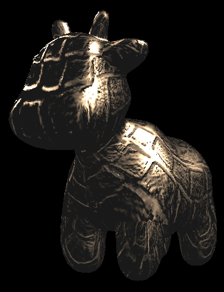
下图是bump_fragment_shader得到的结果：

Displacement shader

同bump mapping，在这里直接搬运别人的代码如下：

Eigen::Vector3f displacement_fragment_shader(const fragment_shader_payload& payload)
{
    
    Eigen::Vector3f ka = Eigen::Vector3f(0.005, 0.005, 0.005);
    Eigen::Vector3f kd = payload.color;
    Eigen::Vector3f ks = Eigen::Vector3f(0.7937, 0.7937, 0.7937);

    auto l1 = light{{20, 20, 20}, {500, 500, 500}};
    auto l2 = light{{-20, 20, 0}, {500, 500, 500}};

    std::vector<light> lights = {l1, l2};
    Eigen::Vector3f amb_light_intensity{10, 10, 10};
    Eigen::Vector3f eye_pos{0, 0, 10};

    float p = 150;

    Eigen::Vector3f color = payload.color; 
    Eigen::Vector3f point = payload.view_pos;
    Eigen::Vector3f normal = payload.normal;

    float kh = 0.2, kn = 0.1;
    
    //
    Vector3f n = normal.normalized();
    float d = sqrt(n.x() * n.x() + n.z() * n.z());
    Vector3f t (n.x() * n.y() / d, d, n.z() * n.y() / d);
    Vector3f b = n.cross(t);

    Matrix3f TBN;
    TBN.col(0) = t, TBN.col(1) = b, TBN.col(2) = n;

    float u = payload.tex_coords.x(), v = payload.tex_coords.y();
    float w = payload.texture->width, h = payload.texture->height;

    float dU = kh * kn * (payload.texture->getColor(u + 1.0f / w, v).norm() - payload.texture->getColor(u, v).norm());
    float dV = kh * kn * (payload.texture->getColor(u, v + 1.0f / h).norm() - payload.texture->getColor(u, v).norm());

    Vector3f ln (-dU, -dV, 1);

    point += (kn * normal * payload.texture->getColor(u, v).norm());
    normal = (TBN * ln).normalized();
    
    Eigen::Vector3f result_color = {0, 0, 0};

    for (auto& light : lights)
    {
        // Calculate the square distance r^2
        float square_distance = (light.position - point).squaredNorm();

        // Calculate the light direction, view direction, normal, and half vector
        Vector3f l = (light.position - point).normalized();
        Vector3f v = (eye_pos - point).normalized();
        Vector3f n = normal.normalized();
        Vector3f h = (l + v).normalized();
        
        // The light intensity
        Vector3f I = light.intensity;

        // Calculate the ambient light, diffuse light and specular light
        Vector3f ambient_light = ka.cwiseProduct(amb_light_intensity);
        Vector3f diffuse_light = kd.cwiseProduct(I / square_distance) * std::max(0.0f, n.dot(l));
        Vector3f specular_light = ks.cwiseProduct(I / square_distance) * std::pow(std::max(0.0f, n.dot(h)), p);

        result_color += ambient_light + diffuse_light + specular_light;
    }

    return result_color * 255.f;
}

可以看到，displacement mapping基本上就是bump mapping + blinn-phong，核心在于通过凹凸贴图改变真实空间中的位置point及其法向量normal，然后再应用常规的blinn-phong着色。

下图是displacement_fragment_shader得到的结果：

通过上面的一系列代码，我们其实能知道，我们的着色频率是Phong Shading，也就是逐像素着色，因为fragment_shader_payload里面存的是每个像素的信息。

Bonus: bilinear interpolation

本次作业的提高题是实现双线性纹理插值，需要首先实现一个新方法Vector3f getColorBilinear(float u, float v)，然后再在shader中调用。

直接在Texture类中增加方法getColorBilinear:

Eigen::Vector3f getColorBilinear (float u, float v)
{
    u = std::fmin(1, std::fmax(u, 0));
    v = std::fmin(1, std::fmax(v, 0));
    
    // The real (u, v) position on texture
    auto u_img = u * width;
    auto v_img = (1 - v) * height;

    // Calculate the nearest four integer coordinates
    float u0 = std::round(u_img - 0.5f);
    float u1 = std::round(u_img + 0.5f); 
    float v0 = std::round(v_img - 0.5f);
    float v1 = std::round(v_img + 0.5f);

    // The interpolation coefficient
    float s = (u_img - u0) / (u1 - u0);
    float t = (v_img - v0) / (v1 - v0);

    auto c00 = image_data.at<cv::Vec3b>(v0, u0);
    auto c01 = image_data.at<cv::Vec3b>(v0, u1);
    auto c10 = image_data.at<cv::Vec3b>(v1, u0);
    auto c11 = image_data.at<cv::Vec3b>(v1, u1);

    auto c0 = c00 + s * (c01 - c00);
    auto c1 = c10 + s * (c11 - c10);

    auto color = c0 + t * (c1 - c0);
    return Eigen::Vector3f(color[0], color[1], color[2]);
}

得到的图片和原来差不太多，有可能是因为纹理图的分辨率还是比较高的。我替换了一张低分辨率的纹理图，得到了下面的两张对比图。注意牛的后腿，显然能发现使用bilinear的更加平滑，这说明bilinear插值能对低分辨率纹理图有比较好的效果。

Summary: the shading pipeline

最后来总结一下我们是怎样实现整个着色过程的：

1. 读取信息：从模型文件中读取Mesh，再从Mesh中加载三角形，及其三个顶点的位置、法线和纹理坐标等其他信息；
2. 顶点处理：分别将顶点变换到view space、projection space和screen space中，保存其中需要的信息；
3. 光栅化：对每个三角形中的每个像素，首先计算出它的重心坐标，然后通过矫正插值计算它在真实空间中的深度、法线、纹理坐标和颜色等信息，最后存入缓存区等待着色；
4. 着色：最后根据不同的着色器按需取出缓存区的信息加以处理，得到一个最终的RGB值，这就是在屏幕上呈现的颜色。

作业四

本次作业非常简单，只需要实现Bézier曲线。

Recursive bézier curve

主要完成的就是两个函数，bezier——循环每个t画出整个曲线，recursive_bezier——对每个t求出对应的点，都不困难。

bezier函数如下：

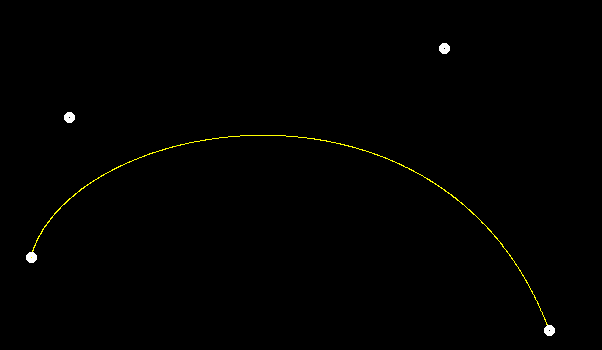
void bezier(const std::vector<cv::Point2f> &control_points, cv::Mat &window) 
{
    float epsilon = 0.001;

    for (float t = 0.0f; t <= 1.0f; t += epsilon)
    {
        auto point = recursive_bezier (control_points, t);
        window.at<cv::Vec3b>(point.y, point.x)[1] = 255;
    }
}

recursive_bezier函数如下：

cv::Point2f recursive_bezier(const std::vector<cv::Point2f> &control_points, float t) 
{
    // Only one point remaining
    if (control_points.size() == 1)
    {
        return control_points[0];
    }
    else 
    {
        // Evaluate new points
        std::vector<cv::Point2f> new_points;
        for (int i = 0; i < control_points.size() - 1; ++i)
        {
            new_points.push_back (control_points[i] + t * (control_points[i + 1] - control_points[i]));
        }
        return recursive_bezier (new_points, t);
    }
}

Using the bernstein polynomial

代码框架提供的Bernstein多项式只能针对四个点，我们把它稍作修改使它支持任意多个点：

void naive_bezier(const std::vector<cv::Point2f> &points, cv::Mat &window) 
{
    // Make this function more generalized
    int n = points.size ();

    for (float t = 0.0; t <= 1.0; t += 0.001) 
    {
        auto point = cv::Point2f(0.0f, 0.0f);

        for (int i = 0; i < n; ++i)
        {
            point += bernstein_polynomial (n - 1, i, t) * points[i];
        }

        window.at<cv::Vec3b>(point.y, point.x)[2] = 255;
    }
}

函数bernstein_polynomial计算对应项的系数：

float bernstein_polynomial (int n, int i, float t)
{
    return recursive_combination (n, i) * std::pow (t, i) * std::pow (1 - t, n - i);
}

函数recursive_combination用于计算组合数：

int recursive_combination (int n, int m)
{
    if (n == 0 || m == 0) return 1;
    return recursive_combination (n, m - 1) * (n - m + 1) / m;
}

这里用到了简单的组合数递推公式：

随便画一画，结果是正确的：

Bonus: antialiasing

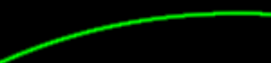
根据作业提示，在着色一个像素的时候，还要根据周围八个像素到当前点的距离去着色这八个点。我们把bezier稍作修改即可：

void bezier(const std::vector<cv::Point2f> &control_points, cv::Mat &window) 
{
    float epsilon = 0.001;

    for (float t = 0.0f; t <= 1.0f; t += epsilon)
    {
        auto point = recursive_bezier (control_points, t);
        window.at<cv::Vec3b>(point.y, point.x)[1] = 255;

        // The actual shading point (x,y)
        int x = point.x;
        int y = point.y;

        // This is used to normalize the color
        float normalization = 3.0f / std::sqrt(2);

        // For each adjacent pixel
        for (int dx = -1; dx <= 1; ++dx)
            for (int dy = -1; dy <= 1; ++dy)
            {   
                // Should be within the bound
                if (x + dx >= 700 || x + dx < 0 || y + dy >= 700 || y + dy < 0)
                    continue;

                // Calculate the distance to the actual shading point
                float distance = cv::norm((point - cv::Point2f(x + dx + 0.5, y + dy + 0.5)));
                // Normalize according to the distance
                float ratio = 1 - distance / normalization;

                // Shading
                window.at<cv::Vec3b> (point.y + dy, point.x + dx)[1] = std::fmax (window.at<cv::Vec3b> (point.y + dy, point.x + dx)[1], 255 * ratio);
            }
    }
}

这里需要注意的是我们对求出来的距离distance进行了归一化，归一化系数normalization是当前着色点到它相邻点的最大距离，也就是。

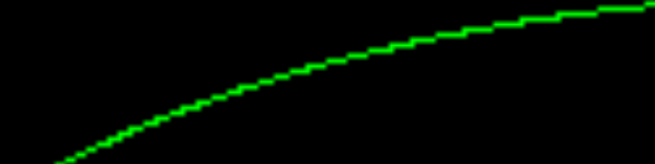
反走样前后对比如下：

作业五

本次作业也非常简单，主要是实现光线投射和光线与三角形相交。

Framework

还是先来大致梳理一下代码框架。

程序从main.cpp开始，首先创建了两个球体sph1和sph2，然后创建了两个三角形，最后创建了两个光源。渲染流程从r.Render(scene)开始。

在开始介绍Render函数之前，先介绍几个接下来要用到的函数。

首先是代码中的reflect函数，它接受一个单位向量I和一个法向量N，返回I关于法向量所定义的平面的镜面反射向量。

第二，是函数refract，它根据Snell's law计算入射光进入某物体后的折射光。它接受三个参数：I是入射光，N是入射点的法向量，ior是折射系数。具体数学就不多展开了。

第三，函数fresnel根据Fresnel equation计算反射率。它接受三个参数：I是入射光，N是入射点的法向量，ior是折射系数。

第四，trace函数求与给定光线发生碰撞的第一个物体。它接受三个参数：orig是光源位置，dir是光线方向，objects是所有待检测的物体。它返回一个存储碰撞信息的结构体hit_payload，主要是光线长度t和碰撞物体hit_obj。

第五，是最关键的castRay函数。它主要做的事情就是它从光源位置orig以方向dir射出一条光线，打到一个碰撞点hitPoint上，又从该点形成一条折射光线和一条反射光线，把这两条光线收到的颜色通过fresnel加起来，就是hitPoint这个点上的颜色hitColor。上述操作递归进行，直到最大深度maxDepth。

所有材质分为三种：

• REFLECTION_AND_REFRACTION: 透明的，既会反射也会折射，它本身没有颜色，表面的颜色来自反射和折射光携带的颜色；
• REFLECTION：纯反射材质，它的颜色来自反射光的颜色；
• DIFFUSE_AND_GLOSSY：它本身有颜色，使用Phong Shading Model计算颜色。在这里，遍历场景中的所有光源，判断对当前光源而言着色点是否在阴影里，如果不在，则计算漫反射光照和镜面反射光照。

现在回到Render函数。它一开始创建了framebuffer，用于记录每个像素的颜色值，然后对每个像素，从屏幕空间投射出一条射线，通过上面的castRay计算得到当前像素的颜色。最后再把这张图存下来。

Render

我们唯一需要实现的就是如何从屏幕空间投射一条射线。回顾我们之前相机的MVP变换：

• Model：变换空间中的物体，这里不涉及；
• View：视图变换，即把相机放到原点，相机看向方向，这里只需要改变eye_pos，那么View矩阵就是
• Perspective：透视投影变换是

最后还有个视口变换：

所以，对于空间中的一个，在经过上述变换后最终的点是：

由于我们不关注，所以不考虑它的值。如此一来，对于屏幕空间中的一个点，我们可以把它映射回三维空间中的点（同样不考虑）：

其中。

所以，此时的点坐标为在，光线方向就是从相机位置到这个点，正好就是。所以eye_pos对于求光线而言并没有作用。

所以，我们立刻能写出下面的代码：

// generate primary ray direction
float x = (2 * (i + 0.5) / scene.width - 1) * scale * imageAspectRatio;
float y = (1 - 2 * (j + 0.5) / scene.height) * scale;

// Don't forget to normalize this direction!
Vector3f dir = normalize(Vector3f(x, y, -1)); 

上面的代码中假定了近平面为。注意取了负，这是因为屏幕空间是以左上角为原点，向下方向为轴正方向的，所以最后得到的值要取负。

Ray intersect with triangle

Proof of the Moller-Trumbore algorithm

这里使用的算法是Moller-Trumbore算法判断光线与三角形相交。即假设光源为，光照射方向为，三角形三个点为,,。如果光线与三角形有交点，那么就可以用重心坐标表示：

这个方程的解如下：

其中，。

我们首先来证明一下这个结论。

对第一个方程稍加整理，就能得到：

写成矩阵形式，有：

记。则有：

显然，这是一个线性方程组，而求解线性方程组最常用的方法是Cramer's Rule。所以，上述线性方程组的解我们可以写出来是：

对于三阶行列式我们不难得到它与叉乘/点乘的关系如下:

所以，我们能够对上式做最后的化简：

最后再令，就得到了最开始的结果。

The rayTriangleIntersect function in Triangle.hpp

根据上面的公式，我们很容易能写出下面的代码：

bool rayTriangleIntersect(const Vector3f& v0, const Vector3f& v1, const Vector3f& v2, const Vector3f& orig, const Vector3f& dir, float& tnear, float& u, float& v)
{
    Vector3f S = orig - v0;
    Vector3f E1 = v1 - v0;
    Vector3f E2 = v2 - v0;
    Vector3f S1 = crossProduct (dir, E2);
    Vector3f S2 = crossProduct (S, E1);
    float S1_dot_E1 = dotProduct (S1, E1);

    tnear = dotProduct (S2, E2) / S1_dot_E1;
    u = dotProduct (S1, S) / S1_dot_E1;
    v = dotProduct (S2, dir) / S1_dot_E1;

    return tnear > 0 && u >= 0 && u <= 1 && v >= 0 && v <= 1 && u + v <= 1;
}

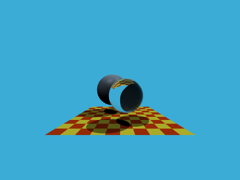
最后生成的图是：

作业六

本节课主要实现Bounding Volume Hierarchy (BVH) 和 Surface Area Heuristic (SAH) 加速结构。代码框架整体上和前一次作业一样，但有些部件进一步进行了拆分。因为上一次作业我完整没有分析代码框架，这次作业按照调用顺序进行分析，在这个过程中完成作业。

Overview of main.cpp

还是从main.cpp开始介绍，作为整个程序的入口。

Initialize the scene, add model and light

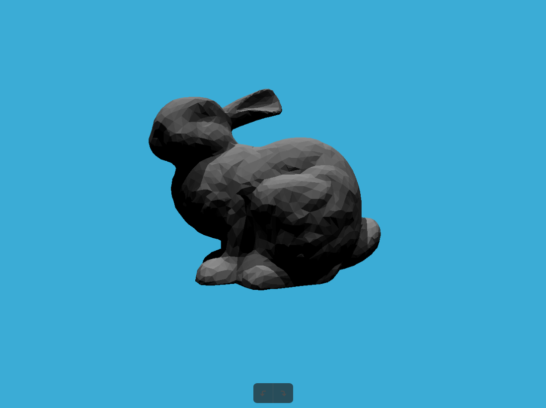
在开头的几行，代码初始化了一个场景，并加载了模型和光照:

Scene scene(1280, 960);

MeshTriangle bunny("../models/bunny/bunny.obj");

scene.Add(&bunny);
scene.Add(std::make_unique<Light>(Vector3f(-20, 70, 20), 1));
scene.Add(std::make_unique<Light>(Vector3f(20, 70, 20), 1));

Initialize BVH and renderer

下面，对场景构造了BVH，并执行整个场景的渲染。BVH和renderer是本次作业的核心。

scene.buildBVH();

Renderer r;

auto start = std::chrono::system_clock::now();
r.Render(scene);
auto stop = std::chrono::system_clock::now();

下面来看下场景包含什么内容。

Scene.hpp and Scene.cpp

Variables and methods

Scene.hpp和Scene.cpp定义了关于场景的high-level参数，包括长宽、fov、背景色、光线弹射的最大深度、场景的BVH、场景中的物体和光源，以及一些必要的函数。

一些关键的函数如下：

• buildBVH: 构建场景的BVH，下面详解。
• intersect: 使用BVH计算与给定光线相交的物体，返回相交点的信息（一个类型为Intersection的结构体），下面详解。
• castRay: 通过光线追踪递归计算某一点的颜色值，与上次作业一样。
• trace: 找到与光线碰撞的最近物体及碰撞点信息，与上次作业一样。
• reflect: 计算反射光线。
• refract: 计算折射光线。
• fresnel: 根据Fresnel equation计算反射率。

Scene::buildBVH and BVHAccel

Scene::buildBVH函数为整个场景构建BVH：

void Scene::buildBVH() {
    printf(" - Generating BVH...\n\n");
    this->bvh = new BVHAccel(objects, 1, BVHAccel::SplitMethod::NAIVE);
}

这是通过创建一个BVHAccel类对象实现的，它接受三个参数：场景中的所有物体primitives，叶子结点最多物体数量maxPrimsInNode，和使用的构造方法splitMethod。构造方法如果是NAIVE则使用中间物体构造BVH，如果是SAH就使用提高题里的SAH构建BVH。这个对象内最终赋值的是一个BVHBuildNode*类型的root变量，表示这个构造的BVH树的根节点。

进入到构造函数内，我们发现它实际上是通过调用BVHAccel::recursiveBuild递归地构建BVH的。这个函数接受一个std::vector<Object*>作为参数，并返回一个BVHBuildNode*类型对象，表示当前的BVH结点。每个BVHBuildNode对象包含一个三维包围盒Bound3，一个同类型的左结点和右结点，还有一个Object*对象，只不过这个Object*只有在当前结点最只包含一个Object时才会被赋值，否则就不会被赋值。

下面开始介绍recursiveBuild函数。一开始首先初始化了一个默认的BVHBuildNode对象：

BVHBuildNode* node = new BVHBuildNode();

然后，遍历所有物体，将所有物体的包围盒合并起来，得到一个包含所有物体的大的包围盒（但实际上这里计算得到的包围盒没有用到，因为每个结点的包围盒可以递归通过求左右子结点包围盒的并集得到）：

Bounds3 bounds;
for (int i = 0; i < objects.size(); ++i)
    bounds = Union(bounds, objects[i]->getBounds());

如果给定的物体只有一个，那么当前结点就是个叶子结点，给BVHBuildNode的所有变量赋值，并返回该结点：

if (objects.size() == 1) {
    // Create leaf _BVHBuildNode_
    node->bounds = objects[0]->getBounds();
    node->object = objects[0];
    node->left = nullptr;
    node->right = nullptr;
    return node;
}

如果给定的物体有两个，那么就把这两个物体分开分别作为左右子结点即可：

else if (objects.size() == 2) {
    node->left = recursiveBuild(std::vector{objects[0]});
    node->right = recursiveBuild(std::vector{objects[1]});

    node->bounds = Union(node->left->bounds, node->right->bounds);
    return node;
}

注意到这里本结点的object并没有被赋值，因为它里面实际上包含了不止一个物体。

如果当前结点包含多于两个物体，那么就按照一定策略划分左右子结点。具体策略是，根据所有物体的包围盒的中心构造一个大的包围盒，然后检查这个大的包围盒在哪一个维度最长，选取最长的那个维度对所有物体进行划分，如下面的代码所示：

Bounds3 centroidBounds;
for (int i = 0; i < objects.size(); ++i)
    centroidBounds =
        Union(centroidBounds, objects[i]->getBounds().Centroid());
int dim = centroidBounds.maxExtent();
switch (dim) {
// Split according to the x-axis
case 0:
    std::sort(objects.begin(), objects.end(), [](auto f1, auto f2) {
        return f1->getBounds().Centroid().x <
                f2->getBounds().Centroid().x;
    });
    break;
// Split according to the y-axis
case 1:
    std::sort(objects.begin(), objects.end(), [](auto f1, auto f2) {
        return f1->getBounds().Centroid().y <
                f2->getBounds().Centroid().y;
    });
    break;
// Split according to the z-axis
case 2:
    std::sort(objects.begin(), objects.end(), [](auto f1, auto f2) {
        return f1->getBounds().Centroid().z <
                f2->getBounds().Centroid().z;
    });
    break;
}

对所有的物体排序之后，数组左侧的物体递归地构建BVH树，并将返回的结点作为当前结点的左子结点；右侧同理：

auto beginning = objects.begin();
auto middling = objects.begin() + (objects.size() / 2);
auto ending = objects.end();

auto leftshapes = std::vector<Object*>(beginning, middling);
auto rightshapes = std::vector<Object*>(middling, ending);

assert(objects.size() == (leftshapes.size() + rightshapes.size()));

node->left = recursiveBuild(leftshapes);
node->right = recursiveBuild(rightshapes);

node->bounds = Union(node->left->bounds, node->right->bounds);

通过上面这种递归的方式，我们能很轻松地构建一个BVH树，树的根节点就是root。

Scene::intersect

Scene::intersect也是通过调用BVH树的Intersect方法实现的：

Intersection Scene::intersect(const Ray &ray) const
{
    return this->bvh->Intersect(ray);
}

而BVHAccel::Intersect则是调用BVHAccel::getIntersection方法实现的：

Intersection BVHAccel::Intersect(const Ray& ray) const
{
    Intersection isect;
    if (!root)
        return isect;
    isect = BVHAccel::getIntersection(root, ray);
    return isect;
}

Implementing BVHAccel::getIntersection

这里的BVHAccel::getIntersection就是我们要实现的方法，它的核心思路是从BVH根节点开始遍历整棵树，直到某个叶子结点找到与光线相交的物体，或者找不到与光线相交的物体：

Intersection BVHAccel::getIntersection(BVHBuildNode* node, const Ray& ray) const
{
    // ray is outside the bounding box
    Vector3f invDir = ray.direction_inv;
    std::array<int, 3> disIsNeg = {int(ray.direction.x > 0), int(ray.direction.y > 0), int(ray.direction.z > 0)};
    if (!node->bounds.IntersectP (ray, invDir, disIsNeg))
        return Intersection();

    // node is a leaf node
    if (node->left == nullptr && node->right == nullptr)
        return node->object->getIntersection(ray);
    
    // node is an inner node
    Intersection leftIntersect = getIntersection(node->left, ray);
    Intersection rightIntersect = getIntersection(node->right, ray);
    return leftIntersect.distance < rightIntersect.distance ? leftIntersect : rightIntersect;
}

这里需要稍加说明的是，类型为MeshTriangle的物体包含了很多个Triangle，但是它本身被视为一个Object对象，所以在main.cpp中我们加载的实际上是一个单个MeshTriangle物体，这个物体内部包含了很多三角形。那么此处调用node->object->getIntersection(ray)实际上调用的是MeshTriangle::getIntersection，而这行代码又调用了MeshTriangle内部的另一个bvh->Intersect函数。所以实际上整个程序执行期间有两个BVH，一个是整个场景的BVH，而另一个是这个MeshTriangle内部的BVH。当我们想要在场景的BVH中检测MeshTriangle与光线的碰撞时，实际上又进入到了MeshTriangle内部的BVH，去检查与里面哪个三角形相交。这一点需要说明下。

上面我们调用了包围盒的函数node->bounds.IntersectP，用来判断某个光线是否和包围盒相交，我们需要实现这个函数。

Implementing Bounds3::IntersectP

Bounds3::IntersectP函数判断一条光线是否与一个包围盒相交，这可以用下面的代码描述：

inline bool Bounds3::IntersectP(const Ray& ray, const Vector3f& invDir,
                                const std::array<int, 3>& dirIsNeg) const
{
    Vector3f t_min = (pMin - ray.origin) * invDir;
    Vector3f t_max = (pMax - ray.origin) * invDir;

    if (t_min.x > t_max.x) std::swap (t_min.x, t_max.x);
    if (t_min.y > t_max.y) std::swap (t_min.y, t_max.y);
    if (t_min.z > t_max.z) std::swap (t_min.z, t_max.z);

    float f_enter = fmax(t_min.x, fmax(t_min.y, t_min.z));
    float f_exit = fmin(t_max.x, fmin(t_max.y, t_max.z));

    return f_enter < f_exit && f_exit > 0;
}

中间的三个if语句是为了保证最小值要小于最大值。

Implementing Triangle::getIntersection

这里还需要实现Triangle::getIntersection，前半部分的代码已经提供了，后面的代码比较简单：

inline Intersection Triangle::getIntersection(Ray ray)
{
    Intersection inter;

    if (dotProduct(ray.direction, normal) > 0)
        return inter;
    double u, v, t_tmp = 0;
    Vector3f pvec = crossProduct(ray.direction, e2); // S1
    double det = dotProduct(e1, pvec);
    if (fabs(det) < EPSILON)
        return inter;

    double det_inv = 1. / det;
    Vector3f tvec = ray.origin - v0;  // S
    u = dotProduct(tvec, pvec) * det_inv;
    if (u < 0 || u > 1)
        return inter;
    Vector3f qvec = crossProduct(tvec, e1);  // S2
    v = dotProduct(ray.direction, qvec) * det_inv;
    if (v < 0 || u + v > 1)
        return inter;
    t_tmp = dotProduct(e2, qvec) * det_inv;

    inter.happened = true;
    inter.distance = t_tmp;
    inter.obj = this;
    inter.m = m;
    inter.normal = normal;
    inter.coords = ray(t_tmp);

    return inter;
}

代码已经提供的部分就是上个作业的Moller-Trumbore算法，得到合法的t_tmp之后把所有相交的信息存储在一个Intersection对象中。注意，Ray实现了()运算符重载，给定一个t值，返回光线传播t后的位置，也就是光线和三角形相交的位置。

Renderer.cpp

Renderer.cpp中唯一的函数是Renderer::Render，其作用就是从每个像素射出光线，也就是调用scene.castRay的函数。这里和上次作业的代码略有差别，但也很容易写出来：

Vector3f dir = normalize(Vector3f(x, y, -1)); 
Ray ray (eye_pos, dir, 0);
framebuffer[m++] = scene.castRay(ray, 0);

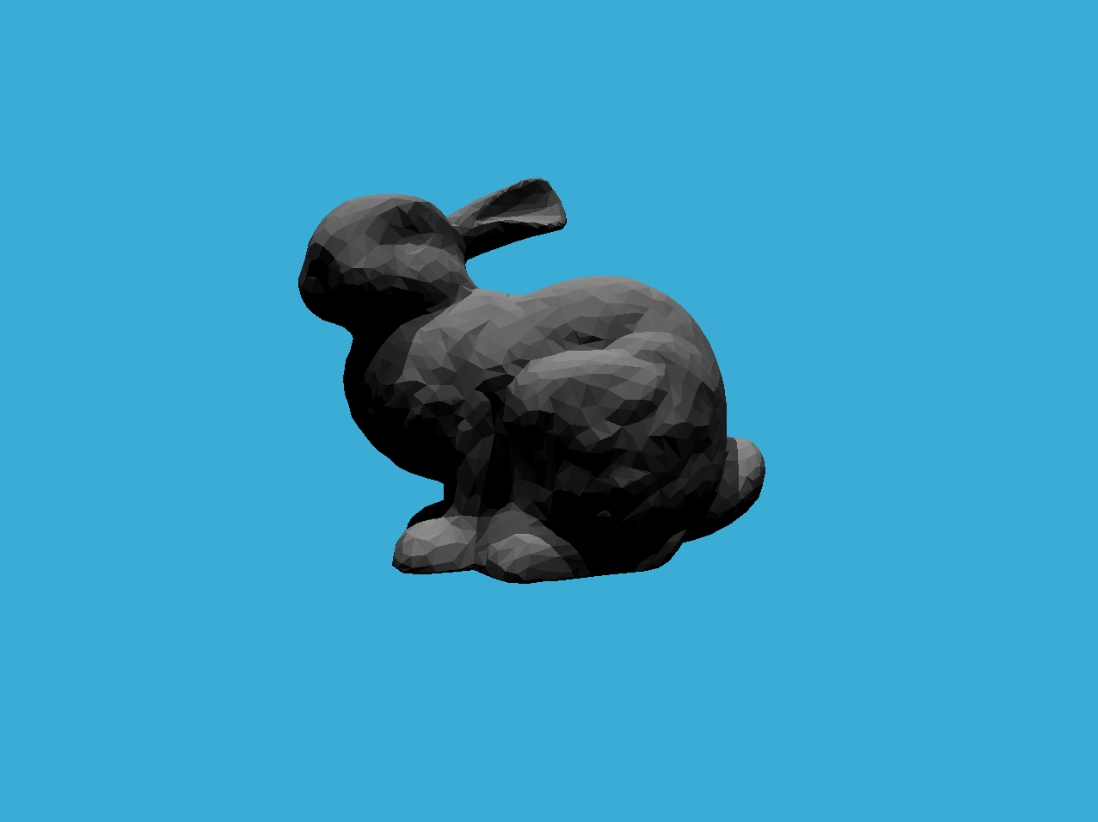
下图是使用BVH执行的结果：

Bonus: Surface Area Heuristic (SAH)

本次作业的提高题是要使用另一种场景加速方法，称为Surface Area Heuristic (SAH)。

Fundamentals of SAH

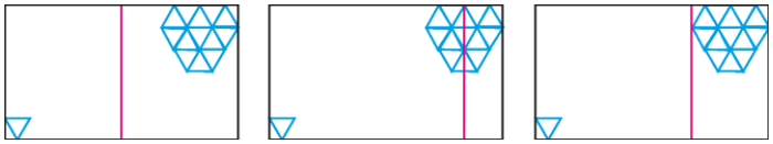
在上面我们构造BVH时，对每个非叶子结点，我们是采取了中间的物体对所有物体划分为左右两个部分。但是这种策略在物体分布及其不均匀的时候是不合理的。

如下图所示，大量的三角形分布在右上角，只有一个三角形分布在左下角。按照我们上面的划分策略，我们会采取第二张图的方法，但是显然，更好的方法是图三，也就是希望越小的包围盒里有越多的物体。这是我们使用SAH的基本想法。

也就是说，SAH是一种划分子结点的方法，对应的是我们上面取中间物体的划分方法。记住，我们的最终目标是找到与光线相交的物体，也就是要尽可能少地遍历树，找到对应物体的叶子结点，那么显然，只有当包围盒里包含更多的物体，或者说相同多的物体被更小的包围盒包围时，才有可能更少地遍历树，因为此时有更大的概率不通过包围盒相交检测。

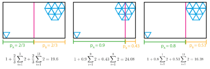
那么怎么才能划分当前结点的物体，让左右两边各自的包围盒更小，同时也能包含更多物体呢？我们可以引入一个经验公式，对每个可能的划分，根据经验公式计算它的划分代价，然后选择代价最小的一个划分作为我们选定的划分。

根据这篇介绍，我们能给出SAH的经验公式如下:

这个公式计算了将当前结点划分为子结点后的代价。其中：

• 是检测光线与两个子包围盒相交所用的时间，以决定选择哪个子结点往下走；
• 是光线进入的概率，也即光线与包围盒相交的概率；
• 是两个子包围盒内包含的物体的数量；
• 是检测光线与物体相交所用的时间。

显然，要让上面式子的值更小，要么让概率更小，要么让包围盒里包含的物体数量更小，当然这两个包围盒的增长趋势是相反的，比如越大，一般就越小，越大，就一定越小。但总的来说，上面的式子是鼓励让更小的包围盒包围尽可能多的物体。

这里我们可以假设为常量，这可以简化计算并且不会带来很大的误差。

最后的问题就是如何计算概率。可以证明，一个凸多面体包含在另一个凸面体中，一个均匀分布的光线在与相交的条件下与相交的概率是它们的表面积之比，即：

这也是SAH名字的由来。

下图是我们假设时，使用SAH进行划分计算得到的值，可以看到，与我们的猜想相符，第三种划分结果最好：

下面我们用代码实现SAH。

Implementing SAH

我们需要重新定义几个函数。

• 函数recursiveBuildSAH类似recursiveBuild，递归地使用SAH构建BVH。

BVHBuildNode* BVHAccel::recursiveBuildSAH(std::vector<Object*> objects)
{
    ...
}

• 函数GetPartition找出所有物体的划分点。

std::size_t BVHAccel::GetPartition (std::vector<Object*> objects, float bucketBorder, int dim)
{
    ...
}

• 函数ComputeCost计算给定划分的Cost。

float BVHAccel::ComputeCost (std::vector<Object*> leftObjects, std::vector<Object*> rightObjects, float t_intersect, float t_traversal)
{
    ...
}

别忘了把它们的函数声明放到BVH.hpp中。

首先来看函数recursiveBuildSAH：

BVHBuildNode* BVHAccel::recursiveBuildSAH(std::vector<Object*> objects)
{
    // Number of buckets
    constexpr int nBuckets = 10;

    // Min and max axis value
    float min_axis, max_axis;

    // Min cost
    float min_cost = std::numeric_limits<float>::max();

    BVHBuildNode* node = new BVHBuildNode();
    // Compute bounds of all primitives in BVH node
    Bounds3 bounds;
    for (int i = 0; i < objects.size(); ++i)
        bounds = Union(bounds, objects[i]->getBounds());
    if (objects.size() == 1) {
        // Create leaf _BVHBuildNode_
        node->bounds = objects[0]->getBounds();
        node->object = objects[0];
        node->left = nullptr;
        node->right = nullptr;
        return node;
    }
    else if (objects.size() == 2) {
        node->left = recursiveBuildSAH(std::vector<Object*>{objects[0]});
        node->right = recursiveBuildSAH(std::vector<Object*>{objects[1]});

        node->bounds = Union(node->left->bounds, node->right->bounds);
        return node;
    }
    else {
        Bounds3 centroidBounds;
        for (int i = 0; i < objects.size(); ++i)
            centroidBounds =
                Union(centroidBounds, objects[i]->getBounds().Centroid());
        int dim = centroidBounds.maxExtent();
        switch (dim) {
        case 0:
            std::sort(objects.begin(), objects.end(), [](auto f1, auto f2) {
                return f1->getBounds().Centroid().x <
                       f2->getBounds().Centroid().x;
            });
            // assign to min_axis and max_axix
            min_axis = (*objects.begin())->getBounds().Centroid().x;
            max_axis = (*--objects.end())->getBounds().Centroid().x;
            break;
        case 1:
            std::sort(objects.begin(), objects.end(), [](auto f1, auto f2) {
                return f1->getBounds().Centroid().y <
                       f2->getBounds().Centroid().y;
            });
            // assign to min_axis and max_axix
            min_axis = (*objects.begin())->getBounds().Centroid().y;
            max_axis = (*--objects.end())->getBounds().Centroid().y;
            break;
        case 2:
            std::sort(objects.begin(), objects.end(), [](auto f1, auto f2) {
                return f1->getBounds().Centroid().z <
                       f2->getBounds().Centroid().z;
            });
            // assign to min_axis and max_axix
            min_axis = (*objects.begin())->getBounds().Centroid().z;
            max_axis = (*--objects.end())->getBounds().Centroid().z;
            break;
        }
/*
        auto beginning = objects.begin();
        auto middling = objects.begin() + (objects.size() / 2);
        auto ending = objects.end();

        auto leftshapes = std::vector<Object*>(beginning, middling);
        auto rightshapes = std::vector<Object*>(middling, ending);

        assert(objects.size() == (leftshapes.size() + rightshapes.size()));

        node->left = recursiveBuild(leftshapes);
        node->right = recursiveBuild(rightshapes);

        node->bounds = Union(node->left->bounds, node->right->bounds);
*/
        std::vector<Object*> leftShapes;
        std::vector<Object*> rightShapes;

        for (int i = 1; i < nBuckets; ++i)
        {
            // iterate through each bucket
            float bucketBorder = min_axis + 1.0f * i / nBuckets * (max_axis - min_axis);
            // the `partition` point of objects
            auto partition = GetPartition (objects, bucketBorder, dim);
            
            // same as recursiveBuild
            auto beginning = objects.begin();
            auto middling = objects.begin() + partition;
            auto ending = objects.end();

            auto leftObjects = std::vector<Object*>(beginning, middling);
            auto rightObjects = std::vector<Object*>(middling, ending);

            // compute cost
            float cost = ComputeCost (leftObjects, rightObjects, 1.0f, 1.0f / 8);
            
            // if lower cost
            if (cost < min_cost)
            {
                min_cost = cost;
                leftShapes = leftObjects;
                rightShapes = rightObjects;
            }
        }
        assert(objects.size() == (leftShapes.size() + rightShapes.size()));

        node->left = recursiveBuildSAH(leftShapes);
        node->right = recursiveBuildSAH(rightShapes);

        node->bounds = Union(node->left->bounds, node->right->bounds);
    }

    return node;
}

前面的大部分内容和recursiveBuild都是一样的，主要的不同是函数开头的变量定义，和最后递归的部分，我把recursiveBuild原来的内容注释掉方便对比。

在函数开头，我们新定义了几个变量：

// Number of buckets
constexpr int nBuckets = 10;

// Min and max axis value
float min_axis, max_axis;

// Min cost
float min_cost = std::numeric_limits<float>::max();

分别是bucket的数量（这里为一个常数10），当前在某个轴上划分的最小值和最大值，和划分的最小Cost。在上面我们分析SAH的时候，我们可以对当前包围盒中的每个物体遍历，每次都取一个物体作为划分点对左右进行划分，计算Cost然后比较，最后找到最小Cost的那次划分作为真正的划分。但显然，当物体很多的时候，这样遍历的效率是很低的。我们采用基于Bucket的划分方法，把当前包围盒均匀地分为若干个Bucket，去遍历每个Bucket的边界而不是每个物体，这样最多只需要枚举Bucket的数量就可以得到最优划分（当然这里的最优不是枚举每个物体意义上的最优），在不显著降低效果的前提下能够大幅提升构建效率。

在当前包围盒只有一个或者两个物体时，采取和函数recursiveBuild一样的做法，而在包含多于两个物体时，就要去找按照哪个轴划分，同时对所有物体排序并得到当前轴上所有物体包围盒中心在所选取轴上的最小最大值，也就是代码中给变量min_axis, max_axis赋值。

最后，就是去枚举每个Bucket。首先得到Bucket的边界：

float bucketBorder = min_axis + 1.0f * i / nBuckets * (max_axis - min_axis);

然后基于边界和所选取的轴对所有物体进行划分，即找到一个分界物体，使得左边的物体的包围盒中心在所选取轴上的值都小于Bucket边界值，右侧物体的包围盒中心在所选取轴上的值都大于Bucket边界值：

auto partition = GetPartition (objects, bucketBorder, dim);

找到边界之后，将所有物体分成两组：

auto beginning = objects.begin();
auto middling = objects.begin() + partition;
auto ending = objects.end();

auto leftObjects = std::vector<Object*>(beginning, middling);
auto rightObjects = std::vector<Object*>(middling, ending);

计算Cost：

float cost = ComputeCost (leftObjects, rightObjects, 1.0f, 1.0f / 8);

如果得到的Cost比当前记录的Cost还要小，则更新最小Cost和当前划分：

if (cost < min_cost)
{
    min_cost = cost;
    leftShapes = leftObjects;
    rightShapes = rightObjects;
}

在枚举完所有的Bucket之后，就得到了最后的划分，递归构建左右子树即可：

assert(objects.size() == (leftShapes.size() + rightShapes.size()));

node->left = recursiveBuildSAH(leftShapes);
node->right = recursiveBuildSAH(rightShapes);

node->bounds = Union(node->left->bounds, node->right->bounds);

函数GetPartition接受已排序的所有物体、Bucket边界值和所选取的轴，返回物体中的一个划分位置：

std::size_t BVHAccel::GetPartition (std::vector<Object*> objects, float bucketBorder, int dim)
{
    for (int i = 0; i < objects.size(); ++i)
    {
        Vector3f centroid = objects[i]->getBounds().Centroid();
        switch (dim)
        {
            case 0:
                if (centroid.x > bucketBorder) 
                    return i;
                break;
            case 1:
                if (centroid.y > bucketBorder) 
                    return i;
                break;
            case 2:
                if (centroid.z > bucketBorder) 
                    return i;
                break;
        }
    }
    return objects.size() - 1;
}

注意到比较大小时是以每个物体包围盒的中心位置为基础的。

函数ComputeCost接受已经划分的左右物体列表，还有两个计算需要的变量t_intersect和t_traversal：

float BVHAccel::ComputeCost (std::vector<Object*> leftObjects, std::vector<Object*> rightObjects, float t_intersect, float t_traversal)
{
    Bounds3 leftBound, rightBound;
    for (int i = 0; i < leftObjects.size(); ++i)
        leftBound = Union(leftBound, leftObjects[i]->getBounds());
    for (int i = 0; i < rightObjects.size(); ++i)
        rightBound = Union(rightBound, rightObjects[i]->getBounds());
    
    Bounds3 currentBound = Union(leftBound, rightBound);

    float pA = leftBound.SurfaceArea() / currentBound.SurfaceArea();
    float pB = rightBound.SurfaceArea() / currentBound.SurfaceArea();

    float cost = t_traversal + pA * leftObjects.size() * t_intersect + pB * rightObjects.size() * t_intersect;
    return cost;
}

Modify other functions

要在本次作业中使用SAH，还要修改几个其他地方。一是在Scene::buildBVH中把构造方法改为SAH：

void Scene::buildBVH() {
    printf(" - Generating BVH...\n\n");
    this->bvh = new BVHAccel(objects, 1, BVHAccel::SplitMethod::SAH);
}

然后在BVHAccel的构造函数中加入判断条件：

if (splitMethod == SplitMethod::NAIVE)
    root = recursiveBuild(primitives);
else
    root = recursiveBuildSAH(primitives);

最后还要在MeshTriangle的构造函数里把内部的BVH构造方法改为SAH：

// bvh = new BVHAccel(ptrs);
bvh = new BVHAccel(ptrs, 1, BVHAccel::SplitMethod::SAH);

下图是使用SAH的效果图：

然后是BVH和SAH的效率对比。为了使NAIVE BVH和SAH BVH效率对比更加突出，我在main.cpp中连续调用了100次r.Render(scene)，然后再看二者所花费的时间。结果如下：

NAIVE:
Time taken: 0 hours
          : 5 minutes
          : 328 seconds

SAH:
Time taken: 0 hours
          : 5 minutes
          : 300 seconds

可以看到，对本次作业而言，SAH还是比NAIVE方法更高效，实际上，对更复杂的模型和场景，SAH的优势会更明显。

Summary

最后来总结一下光线追踪的流程：

1. 加载场景中的所有物体，包括顶点位置、材质、材质坐标、法线等等；
2. 构建BVH，可以使用NAIVE方法或者SAH方法，NAIVE方法是选取当前包围盒所包含物体的中间物体作为划分点，而SAH方法是选择使得Cost最小的物体作为划分点，基本思想是让更小的包围盒包围更多的物体；
3. 执行光追，从相机向每个像素发出光线，使用BVH找到最近的交点，递归地得到该点的颜色；
4. 将颜色绘制在每个像素上。

作业七

本次作业将实现完整的Path Tracing算法。

Transfer code

Triangle::getIntersection

与上次作业一样：

inter.happened = true;
inter.distance = t_tmp;
inter.obj = this;
inter.m = m;
inter.normal = normal;
inter.coords = ray(t_tmp);

Bounds3::IntersectP

与上次作业基本一样:

Vector3f t_min = (pMin - ray.origin) * invDir;
Vector3f t_max = (pMax - ray.origin) * invDir;

if (t_min.x > t_max.x) std::swap (t_min.x, t_max.x);
if (t_min.y > t_max.y) std::swap (t_min.y, t_max.y);
if (t_min.z > t_max.z) std::swap (t_min.z, t_max.z);

float f_enter = fmax(t_min.x, fmax(t_min.y, t_min.z));
float f_exit = fmin(t_max.x, fmin(t_max.y, t_max.z));

return f_enter <= f_exit && f_exit >= 0;

但这里一定要加上等号=，因为存在浮点误差。如果不加等号，画面的大部分内容将为黑色。

BVHAccel::getIntersection

与上次作业一样：

// ray is outside the bounding box
Vector3f invDir = ray.direction_inv;
std::array<int, 3> disIsNeg = {int(ray.direction.x > 0), int(ray.direction.y > 0), int(ray.direction.z > 0)};
if (!node->bounds.IntersectP (ray, invDir, disIsNeg))
    return Intersection();

// node is a leaf node
if (node->left == nullptr && node->right == nullptr)
    return node->object->getIntersection(ray);

// node is an inner node
Intersection leftIntersect = getIntersection(node->left, ray);
Intersection rightIntersect = getIntersection(node->right, ray);
return leftIntersect.distance < rightIntersect.distance ? leftIntersect : rightIntersect;

main.cpp

现在还是根据程序的调用顺序分析一下代码的框架。代码的大部分内容和上次作业一样，不同的地方详解，其他的地方简要说明。

首先仍然是构造场景，然后初始化了三个颜色red, green, white和一个光源light，并定义了它们的漫反射系数Kd。其次加载了若干模型，并加载到场景中。最后构建BVH开始渲染。

Material.hpp

Material.hpp和上次作业有较大差别，这里稍微说明下。

Material中的成员变量包括：

• m_type: 材质类型，当前只有DIFFUSE类型；
• m_emission: 自己向外发出的光；
• ior: 折射率；
• Kd, Ks: 漫反射系数和反射系数；
• specularExponent: 反射指数

新增了三个成员函数：

• sample(const Vector3f &wi, const Vector3f &N): 给定法线N和入射光wi，均匀地在半球上采样一条出射光，因为是均匀采样，所以入射光没有用；
• pdf(const Vector3f &wi, const Vector3f &wo, const Vector3f &N): 给定入射光、出射光和法线，计算其概率密度函数，但由于这里是均匀采样，所以结果恒定为；
• eval(const Vector3f &wi, const Vector3f &wo, const Vector3f &N): 给定入射光、出射光和法线，计算其对应的BRDF，在采样均匀的假设下，这个值恒定为，这里的就是漫反射系数Kd，或者称为albedo。

所以，material实际上定义了一个物体应该被如何着色，它和物体本身的形状、大小没有直接关系。

Scene.cpp

Scene.cpp包含了本次作业需要实现的核心函数，需要稍加分析。

The sampleLight function

sampleLight函数从面光源处采样一个光源。

首先需要说明，本次作业的Object, Sphere, Triangle, MeshTriangle, BVH都增加了一个成员变量area表示面光源的面积，和一个Sample的成员方法表示从面光源从采样一条光线。现在先知道这件事，下面会详细说明。

sampleLight代码如下：

void Scene::sampleLight(Intersection &pos, float &pdf) const
{
    float emit_area_sum = 0;
    for (uint32_t k = 0; k < objects.size(); ++k) {
        if (objects[k]->hasEmit()){
            emit_area_sum += objects[k]->getArea();
        }
    }
    float p = get_random_float() * emit_area_sum;
    emit_area_sum = 0;
    for (uint32_t k = 0; k < objects.size(); ++k) {
        if (objects[k]->hasEmit()){
            emit_area_sum += objects[k]->getArea();
            if (p <= emit_area_sum){
                objects[k]->Sample(pos, pdf);
                break;
            }
        }
    }
}

首先，遍历场景中的所有物体，如果该物体自己是发光的（也就是自己是光源），则把它的光源面积加起来。然后，采样一个数值，找到对应的那个光源，并从这个光源中采样光线，更新发光点的信息pos和概率密度函数pdf。

The castRay function

本次作业主要需要实现的函数是castRay函数，核心思路是从光源和相交点两个层面去采样，前者表示直接光照，后者表示间接关照。这二者的渲染方程分别为：

按照课上讲的内容和作业中的提示，我们不难写出下面的代码：

Vector3f Scene::castRay(const Ray &ray, int depth) const
{
    //
    // Part 1: check if the ray collides with something
    //
    Intersection inter = intersect(ray);
    // If not, there is no light coming in
    if (!inter.happened) return Vector3f();
    // If hitting a light, return the light emission
    if (inter.m->hasEmission()) return inter.m->getEmission();
    //
    // Part 2: sample light (direct light)
    //
    // Define variables
    Vector3f l_dir;
    Intersection lightPos;
    float lightPdf = 0.0f;

    // Sample light, now `lightPos` stores the light pos information
    sampleLight (lightPos, lightPdf);
    // Calculate the inter-to-light direction
    Vector3f toLightDir = (lightPos.coords - inter.coords).normalized();
    // Calculate the distance
    float toLightDisSquare = (lightPos.coords - inter.coords).squareNorm();

    // Check if the ray collides with something else except the light
    Ray toLightRay (inter.coords, toLightDir);
    Intersection interBeforeLight = intersect(toLightRay);
    // Does not collision!
    if (std::sqrt(toLightDisSquare) - interBeforeLight.distance < EPSILON)
    {
        // Calculate the directional light
        l_dir = lightPos.emit * inter.m->eval(toLightDir, -ray.direction, inter.normal) * dotProduct(toLightDir, inter.normal) * dotProduct(-toLightDir, lightPos.normal) / toLightDisSquare / lightPdf;  
    }
    //
    // Part 3: sample ray from intersection (indirect light)
    //
    // Define variables
    Vector3f l_indir;

    // Russian Roulette test
    if (get_random_float() > RussianRoulette) return l_dir;
    // Get a sample ray
    Vector3f sampledDir = inter.m->sample(ray.direction, inter.normal).normalized();
    Ray sampledRay (inter.coords, sampledDir);
    // Intersection test
    Intersection sampleInter = intersect(sampledRay);
    // If ray hits a non-emitting object
    if (sampleInter.happened && !sampleInter.m->hasEmission())
    {
        float pdf = inter.m->pdf(ray.direction, sampledDir, inter.normal);
        l_indir = castRay(sampledRay, depth + 1) * inter.m->eval(sampledDir, -ray.direction, inter.normal) * dotProduct(sampledDir, inter.normal) / pdf / RussianRoulette;
    }

    return l_dir + l_indir;
}

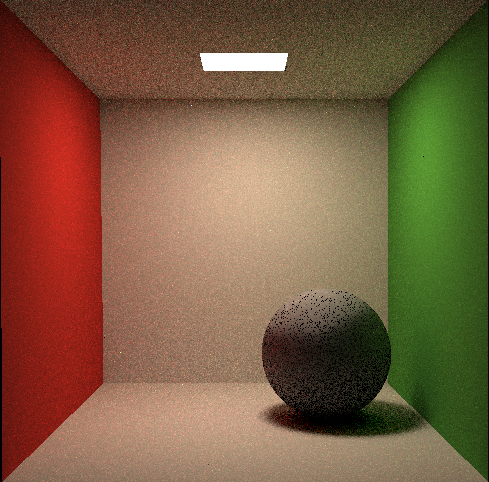
代码里添加了注释帮助理解。整体流程是比较清楚的：首先当前光线检查是否和场景中的物体相交，如果相交，是否是光源，则说明该位置可以直接被光源照射，此时返回光源的颜色即可；然后计算直接光照，从光源采样光线，计算光线打到相交点接受的能量有多少，注意要检查采样的光线到相交点之间是否有阻挡；第三步计算间接光照，从相交点随机采样一条向外的光线，打到一个非光源物体上，递归地计算该光线接受到的能量；最后把直接光和间接光相加即可。

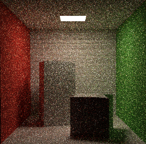
这里需要理解一点：为什么间接光照要检查是非发光物体。这是因为如果不考虑是否发光，那么当光线打到发光物体时，相当于是计算了两次直接光照，最后得到的画面会很奇怪。如下图所示：

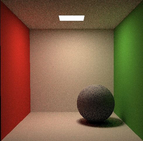
你还会注意到，背后的墙上有很多黑色的横向条纹，这是因为背面墙的颜色基本都来自顶上光源的直接光照，而在计算直接光照的时候我们判定了它们之间是否有阻挡，即std::sqrt(toLightDisSquare) - interBeforeLight.distance < EPSILON，这里的EPSILON在原始代码中很小，这就会因精度问题将其误判为中间存在阻挡。所以，只要把EPSILON稍微调大点即可。

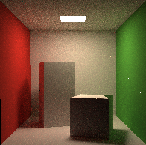
下图是设置EPSILON=0.001并在计算间接光照时判断是否为发光体时生成的结果：

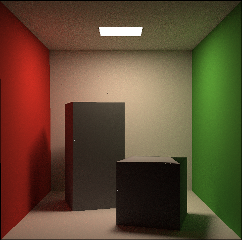
上面都设置SPP=10，所以你会看到噪点比较多。下面是设置SPP=128时的结果：

所用的时间是：

Time taken: 1 hours
          : 100 minutes
          : 6004 seconds

The Sample function

上面的代码需要进一步解释的是如何采样面光源，也就是sampleLight里使用到的函数。

What is area

首先要明确，area代表的是什么？在给定的代码中，所有的物体都表示为MeshTriangle，而一个MeshTriangle是由若干个Triangle组成的，在MeshTriangle的构造函数中，我们发现它的area是内部每个Triangle的area之和：

for (auto& tri : triangles){
    ptrs.push_back(&tri);
    area += tri.area;
}

而每个Triangle的area在构造时已经给出了：

area = crossProduct(e1, e2).norm()*0.5f;

这就是三角形的面积。所以，area代表的就是整个物体的表面积。

The Sample function in Sphere.hpp

有了整个面光源的表面积，我们就可以采样一条光线了。对不同的物体，采样的方式略有差别，我们先来看球型的面光源如何采样。

void Sample(Intersection &pos, float &pdf){
    float theta = 2.0 * M_PI * get_random_float(), phi = M_PI * get_random_float();
    Vector3f dir(std::cos(phi), std::sin(phi)*std::cos(theta), std::sin(phi)*std::sin(theta));
    pos.coords = center + radius * dir;
    pos.normal = dir;
    pos.emit = m->getEmission();
    pdf = 1.0f / area;
}

首先随机得到一个和，然后就能得到一个随机方向dir，从而就能得到球面上一个随机的坐标coords，这就是采样的光线的位置。然后设置法线方向normal、光强度emit和概率密度pdf。

The Sample function in Triangle.hpp

再来看三角形如何采样：

void Sample(Intersection &pos, float &pdf){
    float x = std::sqrt(get_random_float()), y = get_random_float();
    pos.coords = v0 * (1.0f - x) + v1 * (x * (1.0f - y)) + v2 * (x * y);
    pos.normal = this->normal;
    pdf = 1.0f / area;
}

首先得到之间随机的两个坐标，然后计算三个值，这三个值加起来为，所以就能在三角形三个顶点中插值，得到的结果就是三角形内的一个随机的点。然后设置normal和pdf即可。

The Sample function in BVH.cpp

对于MeshTriangle类型的物体，需要首先随机采样一个三角形，然后再按照上面三角形采样的方法进行即可。对于随机采样三角形，首先随机得到一个面积p，然后使用BVH去找到对应的三角形即可。注意，这一行代码pdf *= node->area是为了把在node->object->Sample(pos, pdf)里改变的pdf还原到1.0f。

void BVHAccel::getSample(BVHBuildNode* node, float p, Intersection &pos, float &pdf){
    if(node->left == nullptr || node->right == nullptr){
        node->object->Sample(pos, pdf);
        pdf *= node->area;
        return;
    }
    if(p < node->left->area) getSample(node->left, p, pos, pdf);
    else getSample(node->right, p - node->left->area, pos, pdf);
}

void BVHAccel::Sample(Intersection &pos, float &pdf){
    float p = std::sqrt(get_random_float()) * root->area;
    getSample(root, p, pos, pdf);
    pdf /= root->area;
}

Bonus: Multi-threading

C++的多线程可以使用std::thread实现，用法可以参考这里。基于此，我们不难写出下面的代码，只需要稍加修改Renderer::Render即可（注意加上头文件#include <thread>）：

void DoThread (const Scene& scene, 
             const float scale, 
             const float imageAspectRatio, 
             const Vector3f eye_pos,
             std::vector<Vector3f>& framebuffer, 
             int start, 
             int end, 
             const int spp)
{
    for (int m = start; m < end; ++m)
    {
        int i_width = m % scene.width;
        int j_height = m / scene.width;

        float x = (2 * (i_width + 0.5) / (float)scene.width - 1) *
                    imageAspectRatio * scale;
        float y = (1 - 2 * (j_height + 0.5) / (float)scene.height) * scale;
        Vector3f dir = normalize(Vector3f(-x, y, 1));
        for (int k = 0; k < spp; k++){
            framebuffer[m] += scene.castRay(Ray(eye_pos, dir), 0) / spp;  
        }
    }
}

void Renderer::Render(const Scene& scene, bool multiThreading)
{
    std::vector<Vector3f> framebuffer(scene.width * scene.height);

    float scale = tan(deg2rad(scene.fov * 0.5));
    float imageAspectRatio = scene.width / (float)scene.height;
    Vector3f eye_pos(278, 273, -800);
    int spp = 128;

    if (!multiThreading)
    {
        int m = 0;
        std::cout << "SPP: " << spp << "\n";
        for (uint32_t j = 0; j < scene.height; ++j) {
            for (uint32_t i = 0; i < scene.width; ++i) {
                // generate primary ray direction
                float x = (2 * (i + 0.5) / (float)scene.width - 1) *
                        imageAspectRatio * scale;
                float y = (1 - 2 * (j + 0.5) / (float)scene.height) * scale;

                Vector3f dir = normalize(Vector3f(-x, y, 1));
                for (int k = 0; k < spp; k++){
                    framebuffer[m] += scene.castRay(Ray(eye_pos, dir), 0) / spp;  
                }
                m++;
            }
            UpdateProgress(j / (float)scene.height);
        }
        UpdateProgress(1.f);
    }
    else
    {
        int num_threads = 64;
        int step = scene.height * scene.width / num_threads;
        std::vector<std::thread> threads;
        for (int i = 0; i < num_threads; ++i)
            threads.push_back(std::thread(DoThread, std::ref(scene), scale, imageAspectRatio, eye_pos, std::ref(framebuffer), i * step, (i + 1) * step, spp));
        for (int i = 0; i < num_threads; ++i)
            threads[i].join();
        UpdateProgress(1.f);
    }

    // save framebuffer to file
    FILE* fp = fopen("binary.ppm", "wb");
    (void)fprintf(fp, "P6\n%d %d\n255\n", scene.width, scene.height);
    for (auto i = 0; i < scene.height * scene.width; ++i) {
        static unsigned char color[3];
        color[0] = (unsigned char)(255 * std::pow(clamp(0, 1, framebuffer[i].x), 0.6f));
        color[1] = (unsigned char)(255 * std::pow(clamp(0, 1, framebuffer[i].y), 0.6f));
        color[2] = (unsigned char)(255 * std::pow(clamp(0, 1, framebuffer[i].z), 0.6f));
        fwrite(color, 1, 3, fp);
    }
    fclose(fp);    
}

整体思路还是比较明确的，首先定义线程数num_threads，然后计算每个线程要处理的像素数量step，其次创建线程列表threads，最后加入队列threads[i].join()。

对每个线程而言，做的事情和之前单线程一样，唯一不同的是每个线程只负责自己那一部分的像素计算，所以只需要计算对应的宽高即可：

int i_width = m % scene.width;
int j_height = m / scene.width;

注意，这里需要修改CMakeLists.txt如下，才能编译成功：

cmake_minimum_required(VERSION 3.10)
project(RayTracing)

set(CMAKE_CXX_STANDARD 17)

set(THREADS_PREFER_PTHREAD_FLAG ON)
find_package(Threads REQUIRED)


add_executable(RayTracing main.cpp Object.hpp Vector.cpp Vector.hpp Sphere.hpp global.hpp Triangle.hpp Scene.cpp
        Scene.hpp Light.hpp AreaLight.hpp BVH.cpp BVH.hpp Bounds3.hpp Ray.hpp Material.hpp Intersection.hpp
        Renderer.cpp Renderer.hpp)

target_link_libraries(RayTracing ${CMAKE_THREAD_LIBS_INIT})

现在，在开64个线程时，SPP=128花的时间只有：

Time taken: 0 hours
          : 27 minutes
          : 1629 seconds

得到的结果和没用多线程时是一样的：

Bonus: Microfacet

根据课上所讲的内容，我们可以得到下面的微表面模型BRDF公式：

其中是Fresnel term，是shadow-masking term，是normal distribution。下面来实现这个公式，具体的公式推导之后会专门出一篇文章介绍。

Implementing the normal distribution

这里使用GGX分布（Trowbridge-Reitz分布），公式如下：

其中是表面的粗糙程度，是法向量，是半程向量。注意，这里的实际上是真正粗糙度的平方，即，一般用户调节的也是。

下面是代码实现：

float Material::normalGGX(const Vector3f &N, const Vector3f &h, const float &roughness)
{
    float alpha = roughness * roughness;
    float alpha_square = alpha * alpha;
    float d = (dotProduct(N, h) * dotProduct(N, h)) * (alpha_square - 1) + 1;

    return alpha_square / std::max(M_PI * d * d, EPS);
}

Implementing the shadow-masking term

这里使用SchlickGGX：

可以写出下面的代码：

float Material::shadowSchlickGGX(const Vector3f &N, const Vector3f &v, const float &roughness)
{
    float r = roughness + 1;
    float k = r * r / 8.0f;
    float dot = dotProduct(N, v);
    return dot / (dot * (1 - k) + k);
}

float Material::shadowSmith(const Vector3f &N, const Vector3f &wi, const Vector3f &wo, const float &roughness)
{
    float G1 = shadowSchlickGGX(N, wi, roughness);
    float G2 = shadowSchlickGGX(N, wo, roughness);
    return G1 * G2;
}

Fresnel项代码框架已经给出，即fresnel(const Vector3f &I, const Vector3f &N, const float &ior, float &kr)。下面我们只需要实现整个BRDF流程即可。

Implementing BRDF

首先按照最开始的公式把几个项结合起来：

Vector3f Material::f_micro(const Vector3f &N, const Vector3f &wi, const Vector3f &wo, const float &ior, float &kr, const float &roughness)
{
    fresnel(wi, N, ior, kr);
    float G = shadowSmith(N, wi, wo, roughness);
    Vector3f h = ((wi + wo) / 2).normalized();
    float D = normalGGX (N, h, roughness);

    Vector3f f = kr * G * D / std::max(4.0f * dotProduct(N, wi) * dotProduct(N, wo), EPS);
    return f;
}

然后我们修改eval函数如下：

Vector3f Material::eval(const Vector3f &wi, const Vector3f &wo, const Vector3f &N){
    switch(m_type){
        case DIFFUSE:
        {
            // calculate the contribution of diffuse model
            float cosalpha = dotProduct(N, wo);
            if (cosalpha > 0.0f) {
                Vector3f diffuse = Kd / M_PI;
                return diffuse;
            }
            else
                return Vector3f(0.0f);
            break;
        }
        case MICROFACET:
        {
            float cosalpha = dotProduct(N, wo);
            if (cosalpha > 0.0f)
            {
                // define variables
                float roughness = 0.8f; // you can change it to whatever you want
                float kr, kd;
                // microfacet BRDF: the ratio of intensity coming from one direction is reflected 
                Vector3f fr = f_micro(N, wi, wo, ior, kr, roughness);
                // diffuse BRDF: constant  
                kd = 1.0f - kr;
                Vector3f fd = 1.0f / M_PI;

                return Ks * fr + Kd * kd * fd;
            }
            else
                return Vector3f(0.0f);
            break;
        }
    }
}

注意最后返回的值是Ks * fr + Kd * kd * fd，这里的fr是微表面镜面反射的BRDF，这里面已经乘了Fresnel项，也就是入射光有多少能量被反射出去，外面的Ks是这个材质在镜面反射时本身会吸收多少能量，所以还要衰减。同理，fd是假设入射光所有能量都被漫反射出去的比例，但是实际上有一部分被镜面反射了，剩下来的部分就是kd * fd，而Kd是材质在漫反射时本身会吸收多少。

最后，在main.cpp里修改物体的材质：

// Create a diffuse material, it does not induce reflection light
Material* material_diffuse =  new Material(DIFFUSE, Vector3f(0.0f));
material_diffuse->Kd = Vector3f(0.725f, 0.71f, 0.68f);
// Create a microfacet material, it has both reflect and diffuse lights
Material* material_microfacet = new Material(MICROFACET, Vector3f(0.0f));
material_microfacet->Kd = Vector3f(0.3f, 0.3f, 0.3f); // lean to red diffuse
material_microfacet->Ks = Vector3f(0.45f, 0.45f, 0.45f); 
material_microfacet->ior = 1.0f;

MeshTriangle floor("../models/cornellbox/floor.obj", white);
MeshTriangle shortbox("../models/cornellbox/shortbox.obj", material_microfacet);
MeshTriangle tallbox("../models/cornellbox/tallbox.obj", material_microfacet);
MeshTriangle left("../models/cornellbox/left.obj", red);
MeshTriangle right("../models/cornellbox/right.obj", green);
MeshTriangle light_("../models/cornellbox/light.obj", light);

在SPP=128下能得到下面的图：

这里两个立方体比较黑是因为反射率设置得比较小，将其增大，即吸收的光越少，可以得到更明亮的结果。

Using sphere to explore the effect of roughness

直观来看，roughness控制了物体表面的粗糙程度，那么它会怎样影响光照呢？下面在场景中添加一个球体，并改变roughness探究其影响。所有实验均设置SPP=32。

在main.cpp中加入一个球并调整材质的Kd和Ks：

Material* material_microfacet = new Material(MICROFACET, Vector3f(0.0f));
material_microfacet->Kd = Vector3f(0.3f, 0.3f, 0.3f); // lean to green diffuse
material_microfacet->Ks = Vector3f(0.5f, 0.5f, 0.5f); 
material_microfacet->ior = 1.1f;

Sphere sphere (Vector3f(150, 100, 300), 100, material_microfacet);
scene.Add(&sphere);

先设置roughness = 0.1f，下图是结果：

再设置roughness = 0.5f：

最后看roughness = 0.95f：

可以看到，roughness越小，高光越集中，否则越分散。粗糙度越接近1，效果越接近漫反射。

Summary

最后，还是按照惯例总结一下加入BRDF的光线追踪算法：

• 对每个像素，采样若干点向场景发出光线，把所有光线得到的值平均起来；
• 对每个光线，计算直接光照和间接光照两个部分：
  • 对于直接光照，从光源中随机采样一个光线，如果没有阻挡，则计算该点收到直接光照的能量；
  • 对于间接光照，从半球随机采样一个向外的光线，如果打到非发光体，则递归地得到从该光线收到的能量；
  • 在计算能量时，使用Microfacet BRDF从镜面反射和漫反射两个角度考虑，公式为： 其中，是材质本身对镜面反射、漫反射的反射率，如果这个值为零，则表示材质会吸收所有颜色的光，那么呈现出来的就是黑色；是根据Fresnel Equation计算得到的有多大比例的能量会被镜面反射、漫反射出去；是理论上有多少能量能被镜面反射、漫反射出去，它们还需要乘以Fresnel系数和材质自身的反射率。注意，这里的是上面不加Fresnel项的结果，这里提到了外面变成了。
• 最后，把直接光照和间接光照加起来，就是这一点在给定入射光线和出射光线时接受到的能量。

作业八

本次作业将实现一个质点弹簧系统。下面按照作业要求依次说明。

Creating rope in rope.cpp

首先需要在rope.cpp中创建绳子对象。每个绳子由num_nodes个质点组成，每两个质点之间有一根弹簧。质点本身有质量、位置以及是否被钉住这样一个属性；每个弹簧包含它连接的两个质点和弹簧系数k。对num_nodes个质点的弹簧，我们需要构造num_nodes个质点和num_nodes - 1个弹簧。

代码如下:

Rope::Rope(Vector2D start, Vector2D end, int num_nodes, float node_mass, float k, vector<int> pinned_nodes)
{
    // TODO (Part 1): Create a rope starting at `start`, ending at `end`, and containing `num_nodes` nodes.
    Vector2D step = (end - start) / (num_nodes - 1);

    vector<Mass *> _masses;
    vector<Spring *> _springs;

    for (int i = 0; i < num_nodes; ++i) {
        Mass* mass = new Mass(start + i * step, node_mass, false);
        _masses.push_back(mass);
    }

    for (int i = 0; i < num_nodes - 1; ++i) {
        Spring* spring = new Spring(_masses[i], _masses[i + 1], k);
        _springs.push_back(spring);
    }

    for (auto &i : pinned_nodes) {
        _masses[i]->pinned = true;
    }

    masses = _masses;
    springs = _springs;
}

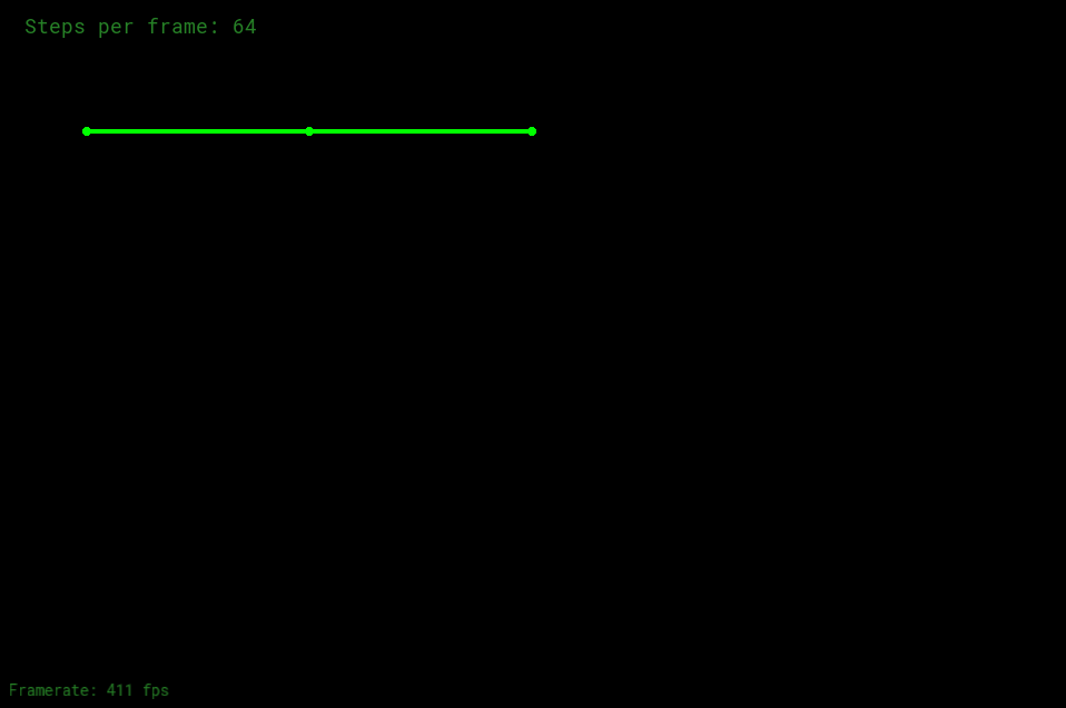
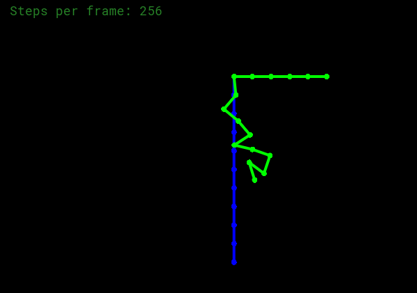
编译之后可以得到下图的结果：

Simulation via euler method

接下来实现显式欧拉和半隐式欧拉方法模拟弹簧运动。胡克定律：

其中是弹簧没有任何拉伸时的长度。

下面是代码：

void Rope::simulateEuler(float delta_t, Vector2D gravity)
{
    for (auto &s : springs)
    {
        // TODO (Part 2): Use Hooke's law to calculate the force on a node
        Vector2D vec = s->m2->position - s->m1->position;
        Vector2D force = -s->k * vec.unit() * (vec.norm() - s->rest_length);

        s->m2->forces += force;
        s->m1->forces += -force;
    }

    for (auto &m : masses)
    {
        if (!m->pinned)
        {
            // TODO (Part 2): Add the force due to gravity, then compute the new velocity and position
            m->forces += gravity * m->mass;

            // TODO (Part 2): Add global damping
            float kd = 0.1;
            m->forces += -kd * m->velocity;

            Vector2D a_t = m->forces / m->mass;

            // Explicit Euler method
            // m->position += m->velocity * delta_t;
            // m->velocity += a_t * delta_t;

            // Semi-implicit Euler method
            m->velocity += a_t * delta_t;
            m->position += m->velocity * delta_t;
        }

        // Reset all forces on each mass
        m->forces = Vector2D(0, 0);
    }
}

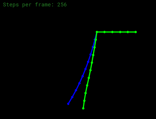
首先对每个弹簧，基于胡克定律累加每个质点的力；然后对每个质点，加上重力，应用全局阻尼，最后更新位置和速度即可。显式欧拉和半隐式欧拉方法的本质区别在于：半隐式欧拉考虑了加速度，因此更加准确。

为了让质点下降的速度慢一些，可以在application.h中把gravity改小一点：

gravity = Vector2D(0, -0.1);

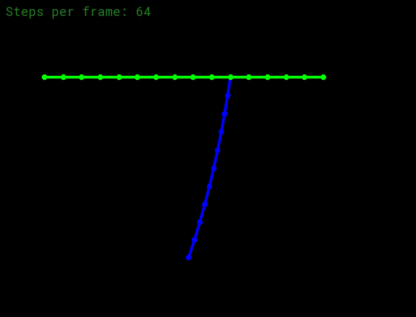
得到的结果如下（蓝色）：

Simulation via Verlet and adding Vetlet damping

使用Verlet模拟，公式如下：

其中是阻尼系数。我们不难写出下面的代码：

void Rope::simulateVerlet(float delta_t, Vector2D gravity)
{
    for (auto &s : springs)
    {
        Vector2D vec = s->m2->position - s->m1->position;
        Vector2D force = -s->k * vec.unit() * (vec.norm() - s->rest_length);

        s->m2->forces += force;
        s->m1->forces += -force;
    }

    for (auto &m : masses)
    {
        if (!m->pinned)
        {
            m->forces += gravity * m->mass;
            Vector2D a_t = m->forces / m->mass;

            Vector2D temp_position = m->position;

            // TODO (Part 3.1): Set the new position of the rope mass
            // TODO (Part 4): Add global Verlet damping
            double damping_factor = 0.00005;

            m->position = m->position + (1 - damping_factor) * (m->position - m->last_position) + a_t * delta_t * delta_t;
            m->last_position = temp_position;
        }
        // Reset all forces on each mass
        m->forces = Vector2D(0, 0);
    }
}

如果我们置，则弹簧永远不会停下来：

如果令，则弹簧能够停止：

至此，我们已完成了GAMES101 所有作业！完结撒花！