Averaging Rotations

Averaging rotations (i.e., quaternions) may not be as simple as you expected. Based on the result of this work, this post goes into the details why a simple weighted average of quaternions does not work and how to implement the real interpolation between quaternions. Part of this post is inspired from Quaternion Weighted Average. Thank Daniel.

Method #1: Simple Weighted Average of Quaternions

Problem Definition

Before I go into the details of today's topic, let me first give a relatively formal definition to the problem I will discuss in the later sections.

(Weighted Average of Rotations) Given a set of rotations (quaternions) and their associated weights where and , we would like to calculate the weighted average rotation such that
(1) is continuous at each with fixed ;
(2) is continuous at each with fixed .

This definition points out for a desired weighted average of rotations, we would like it to maintain robust to slight changes of any of the sub-rotations and to slight changes of weights. As we will see soon, however, most popular solutions do not adhere to these two properties, and thus creating the so-called jump rotation phenomenon.

N-lerp: Normalized Arithmetic Average

N-lerp is short for Normalized Interpolation. It's a widely-used, simple quaterion interpolation strategy to blend multiple quaternions. Basically, an N-lerped quaternion can be calculated as:

The norm at the denominator is necessary to make sure is a unit quaternion, thus representing a rotation.

To see what's wrong with the simple N-lerp method, let's look at simple case.

Assume we are interpolating two quaternions, one is a fixed identity quaternion, i.e., . The second is a quaternion simply rotating around the axis, i.e., the world up direction. But in the following examples, the rotation axis of will slightly deviate from the world up direction so as to let you see how the rotation axis and angle will change as rotation changes. We also set .

As a result, the final interpolated quaternion will be:

The pesudo code is given as follows:

FQuat WeightedQuat = Weights[0] * Cameras[0]->GetActorQuat() + Weights[1] * Cameras[1]->GetActorQuat();;
WeightedQuat.Normalize();

// Get rotation axis and angle of the second rotation
FVector Axis;
float Angle;
Cameras[1]->GetActorQuat().ToAxisAndAngle(Axis, Angle);

PrintString("Rotation Axis is: " + Axis + ", Rotation Angle is: " + Angle + ", w is: " + Cameras[1]->GetActorQuat().W);

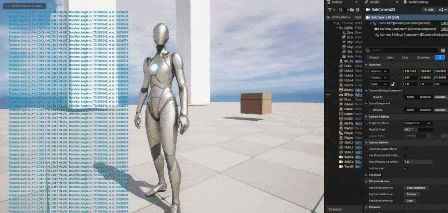
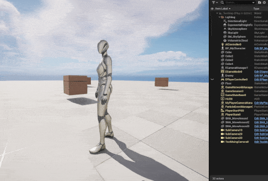
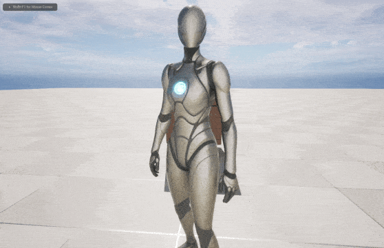
The right panel shows the rotation of the second quaternion, which represents a camera always looking at the cube from the player's view. I also print 's rotation axis and angle, along with its component (real part of the quaternion).

We can see that, when the rotation angle is in , the rotation axis is just the world up direction (as I said, with slight deviation) , which can be justified by the z value printed on screen. However, when the rotation angle surpasses , the rotation axis suddenly flips over to the inverse world up direction, as shown by the negative z value. This means that, when the rotation angle is between , the rotation axis will be flipped and the interpolated quaternion will lie in the other half space of the plane.

The following figure shows what is means to say the other half space of the plane.

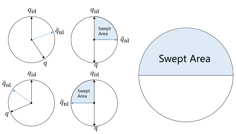
When rotation angle is in , sweeps through the top right quarter of the plane, and when rotation angle is in , sweeps through the top left quarter of the plane. Merging both, only the top half space of the plane will be covered by . The bottom half space, will never have the chance to reach. This is where the jump rotation comes from: the jump change of the rotation axis changes the direction the quaternion is interpolated, and thus changes the final interpolated quaternion.

You may ask, why does the rotation axis have to be flipped? Can you just maintain the rotation axis and let the rotation angle span ? Good question! But it will still cause jump rotation at where angle or , in which case the interpolated quaternion will only span the right half space of the plane. The same problem again.

In fact, we can take a closer look at the the we compute . Let's try to derive a closed form of it.

Assume and , where is the rotation angle of quaternion . In the simple case above, , but in fact it can be any unit rotation axis.

Then we have the following derivations:

The final quaternion spans over half of the rotation range of , meaning that it either spans over if , or spans if . This is exactly what we can expect from what we've discussed above.

This can be easily extended to multiple quaternions. More quaternions there are, more prone to slight changes the average quaternion will be.

S-lerp: Spherical Average

If you are familiar with spherical interpolation (S-lerp), you may wonder if it's possible to maintain continuity using S-lerp. Unfortunately, the jump rotation issue will still arise even if you use S-lerp.

Let's use the same example of N-lerp. The first quaternion is , and assume the second quaternion as . The weights are for both and . By the definition of S-lerp (I use the vanilla S-lerp definition for simplicity), we have the S-lerped quaternion :

This result is equivalent to N-lerp, which is not surprising as S-lerp is still manipulating raw quaternions.

We can use the following figure to illustrate why N-lerp and S-lerp are not working in our trivial case:

The angle of the result quaternion is a periodic function with respect to the rotation angle of . Though we stipulate that angle is within , we can actually extend it to by adding a period of . But in the game engine, the value will be reduced into . It's clear that at the point of , the function is discontinuous, i.e., while , and this therefore causes the jump rotation issue.

Discontinuity of N-lerp

In this section, I will go deeper into the mathematical details of the jump rotation problem, formally proving that simple weighted average with either N-lerp or S-lerp will sometimes (and when) cause the jump rotation problem. This can help us determine in which situations you can safely use N-lerp or S-lerp to average quaternions.

Theorem 1: Quaternion Discontinuity of N-lerp

First, we present a lemma, and it will be used to introduce our theorem.

Lemma 1.1: Given two quaternions and their weights , their N-lerp average quaternion , which is a function of , is discontinuous at rotation angle when , assuming the range angle is where also represents zero rotation.

To prove this lemma, we first rewrite the quaternions as . Then, their weighted average is:

and its norm is:

which gives the explicit expression of :

If is continuous at , or , then it must satisfy that:

with any given and .

We only need to compare to the real part of :

Taking square on both sides and simplifying the equation, we have:

implying that the equality holds only when or or . The solution of is discarded by substituting into the equation above. When or , both sides represent the identity quaternion.

In other words, if , this equation does not hold, and thus, is not continuos at .

We can actually estimate the difference of angle between and . This gives us an intuitive impression of to which extent the rotation will jump. For ease of computation, we take the difference of the squared real parts:

where and are respectively the half rotation angle of quaternion formed by substituting and . Assuming , the above equation simplifies to:

This means that the magnitude of rotation jump is related to the cosine of .

Theorem 1: Given quaternions and their where and , the N-lerp average quaternion , which is a function of , has discontinuous at angle when the rotation angle of quaternion is not , assuming the range angle is where also represents zero rotation.

This can be seen by decomposing to:

Applying Lemma 1.1, Theorem 1 is obvious.

Theorem 1 tells us that the N-lerp style average quaternion will be discontinuous at least at , where quaternion suddenly changes its rotation angle from . For most cases, you cannot make sure the quaternion formed by other sub-quaternions has a rotation angle of zero, so you need to do something to relax Theorem 1 so that there will be less chance for to jump rotate.

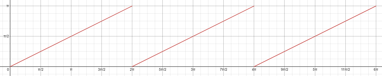
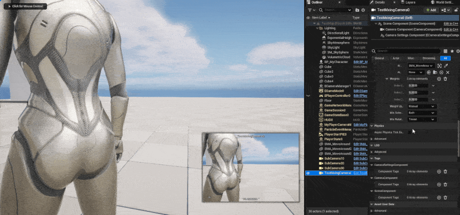
The following figure show us how Theorem 1 performs in practice. Note that in Unreal Engine, the rotation angle range is , so you will see jump rotation at angle rather than we discussed above.

Theorem 2: Weight Discontinuity of N-lerp

Under certain conditions, the average quaternion derived from N-lerp also suffers from discontinuity at particular weight values. We first present the following lemma.

Lemma 2.1: Given two quaternions and their weights , their N-lerp average quaternion , which is function of , is discontinuous at if:
(1) and where ;
(2) and where or .

First we can express as:

and its norm is:

Therefore the explicit form of is:

Considering the real part of :

We then discuss two cases whether or not .

When , we have:

When , it's equivalent to zero and thus is continuous on . To find its discontinuity, we first note that is bounded in as is a quaternion, i.e., a four-dimensional unit vector. Both the denominator and the numerator increase linearly with respect to but at different rates. The only possibility of discontinuity is at some such that , and when traverses from to , the sign of changes.

Let's expand :

which implies:

Through the first and the second equations, we have solutions or . But only the second solution is valid, which applies to all and .

Substituting back into we have:

The proof for the second condition is quite similar. Suppose , we have the following three equations hold:

where . From the first and the second equations, we have two solutions, one is and the other is . Substituting into the third equation, we have three solutions: or or , but none of them give us discontinuity. However, by substituting into the third equation, we have:

Since , the only possible solution is , at which time , and at which time .

Theorem 2: Given quaternions and their weights where and , the N-lerp average quaternion , which is function of , is discontinuous at if:
(1) and where ;
(2) and where or .
where the last quaternions form a new quaternion .

This theorem is obvious when we rewrite as:

The following figure shows that even if sub-quaternions are fixed, changing their weights could also drastically change the final average quaternion, resulting in the jump rotation issue.

Method #2: Matrix Decomposition for the Largest Eigen-value

The jump rotation problem is rooted in the double cover property of quaternions, i.e., and represent the same rotation, so that quaternions provide a 2:1 mapping of the rotation group. Ideally, changing the sign of should not change the result average, but as we've observed above, it indeed changes the result, which is not what we would want.

We would like a way, serving as a 1:1 mapping to the rotation group, to help us disambiguate from the double cover issue. Matrix, does serve this purpose!

Special Orthogonal Matrix Is 1:1 Mapping to Rotation

First according to Wikipedia, we call the subgroup of orthogonal matrices with determinant +1 the special orthogonal group, denoted by . Then we can easily see that every rotation can be represented uniquely by a matrix . This can be proved by showing that any rotation is a linear transformation of the standard basis , which can be represented by a matrix in . For the inverse, any matrix forms a unique orthonormal basis representing a unique rotation upon the standard basis.

Next, we prove that the group of quaternions is 2:1 mapping to . This is obvious because the matrix presentation of a quaternion is:

This is a rotation around vector by a angle of with . It's clear that both and are mapped to .

We can comprehend quaternions as the process of rotation, whereas conceive matrices as the result of rotation, represented as the basis after rotation.

Problem Reformulation

Till now, the problem becomes: given a set of rotation matrices and their associated weights, how do we compute the average rotation? We can first give a particular definition of average: the average rotation should minimize a weighted sum of the squared Frobenius norms of the rotation matrices. This definition can be formulated as follows:

Based on this definition, we can derive a very neat closed form of , which maintains a nice property of continuity of interest. I call this method, M-lerp, short for Matrix Interpolation for rotations, and call the final quaternion as .

In the next subsection, I will go into the details of deriving step by step, basically following this work, but with more elaborations on some of the missing steps.

Solving the Problem

Let's first expand in the form of matrices:

In order to expand , we can rewrite into , assuming any quaternion . Note that is the cross-product matrix:

We can then expand as follows:

From this third equality, we know that .

From the definition of and the expansion of , we can reduce to:

To compute , we have:

which means .

Combining all of these, we have:

Finally, the problem reduces to:

and this corresponds to finding the eigenvector of the largest eigenvalue of .

We can further examine the error quaternion between and , represented by , where is the angle difference between and . On the other hand, can also be interpreted in the form of matrix . Hence,

This implies that the average quaternion that minimizes the weighted sum of Frobenius norms actually minimizes the weighted sum of squared sines of half angles, which is quite intuitive to interpret .

Pseudo Code

There are plenty of algorithms to compute the largest eigenvalue of a symmetric matrix, but the most commonly used one is power iteration, as it's simple to implement and fast in most cases.

I won't go into the details of power iteration. You can easily understand this algorithm with basic linear algebra knowledge.

Giving a set of quaternions and their normalized weights , we can compute the average quaternion as follows:

FQuat AverageQuats(TArray<FQuat>& Quats, TArray<float>& Weights)
{
    FMatrix M = FMatrix(
        0, 0, 0, 0,
        0, 0, 0, 0,
        0, 0, 0, 0,
        0, 0, 0, 0
    );

    for (int i = 0; i < Quats.Num(); ++i)
    {
        FQuat Q = Quats[i];

        M += Weights[i] * FMatrix(
            Q.X * Q.X, Q.X * Q.Y, Q.X * Q.Z, Q.X * Q.W,
            Q.Y * Q.X, Q.Y * Q.Y, Q.Y * Q.Z, Q.Y * Q.W,
            Q.Z * Q.X, Q.Z * Q.Y, Q.Z * Q.Z, Q.Z * Q.W,
            Q.W * Q.X, Q.W * Q.Y, Q.W * Q.Z, Q.W * Q.W
        );
    }

    FVector4 V = PowerIteration(M, FVector(0, 0, 0, 1), 64);
    FQuat Result = FQuat(V.X, V.Y, Y.Z, Y.W);

    return Result;
}

FVector4 PowerIteration(FMatrix& M, FVector4& Init, int Steps, float Eps = 1e-5f)
{
    FVector4 EigenVector = Init;
    float EigenValue = M.Product(EigenVector).X / EigenVector.X;

    for (int i = 0; i < Steps; i++)
    {
        FVector NextVector = M.Product(EigenVector);
        NextVector = NextVector.Normalize();
        NextValue = M.Product(NextVector).X / NextVector.X;

        if (FMath::Abs(EigenValue - NextValue) < Eps)
        {
            break;
        }

        EigenVector = NextVector;
        EigenValue = NextValue;
    }

    return EigenVector;
}

Discontinuity of M-lerp

However, M-lerp does not provide continuity on either. Before going into analysis why and when M-lerp is not working, I give a very simple example to illustrate why M-lerp does not necessarily provide continuity.

Assume and . That is, is the identify rotation and is a rotation around the world up axis by angle .

Optimization goal:

can be calculated as:

Then calculate its eigenvalues:

There are three different eigenvalues: and . The aboslute operator is taken away because

The largest eigenvalue is , and we then calculate its eigenvector:

We can only focus on when , which is when or .

We can respectively take limits for both and :

Since the length of must be one to be a valid quaternion, we have:

This means the result quaternion is not continuous at .

Theorem 3: Quaternion Discontinuity of M-lerp

Theorem 4: Weight Discontinuity of M-lerp

Why Is M-lerp Working

NOTE: When reviewing this section, I find the proofs of Theorem 3 and Theorem 4 are NOT correct. Therefore, M-lerp does NOT ensure continuity for either each rotation or each weight. The incorrect proofs are still left below for reference.

Using the same notion of continuity, we conclude that the matrix decomposition method quite well maintains the property of continuity. This can be formalized as the following theorems.

Theorem 3: Quaternion Continuity of M-lerp

Without loss of generality, we view as a function of , i.e., where . We will show that this function is continuous on .

For ease of illustration, we rewrite as where all variables are fixed except . Then, the average quaternion will be .

We first show that the mapping from a real symmetric matrix to its largest eigenvalue is continuous.

Lemma 3.1: The mapping from a real symmetric matrix to its largest eigenvalue is continuous.

We begin with that fact that the spectral norm of is given by its largest singular value, which is the square root of the largest eigenvalue of . Since is symmetric, we have , and its largest eigenvalue is the squared largest eigenvalue of , and thus the spectral norm of is 's largest eigenvalue.

On the other hand, we know that the spectral norm map is continuous, and thus the map is continuous.

Then, we prove the following lemma.

Lemma 3.2: The mapping from a unit vector to matrix is continuous regarding the Frobenius norm.

Assume is any unit vector and . For and close enough to (in terms of the angle between and ):

As long as , , which proves that the mapping is continuous.

Corollary 3.1: The mapping from a unit vector to matrix is continuous regarding the Frobenius norm, where are fixed coefficients and are fixed unit vectors.

Lemma 3.3: The mapping from a unit vector to the eigenvector of the largest eigenvalue of is continuous. That is, is continuous, where .

In fact, the matrix has only one non-zero eigenvalue, 1, and its eigenvector is . Proof is quite simple:

This means the eigenvector is proportional to . Then, assume and we have:

and any vector parallel to is the eigenvector. For simplicity, we take as the eigenvector. This ends our proof.

Theorem 3: The mapping from a quaternion (4-dimensional unit vector) to the eigenvector of the largest eigenvalue of matrix is continuous.

For ease of elaboration, we rewrite . For any quaternion and close enough quaternion (in terms of their angle ), we know from Lemma 3.1 and Corollary 3.1 that:

where is the largest eigenvalue of and is the largest eigenvalue of . It follows that:

where and are respectively the eigenvector of and , i.e., and .

Since is close enough to , then from Lemma 3.2, there exists a matrix such that and .

On the other hand, we use a rotation matrix to represent the rotation from to , i.e., . Note that is a rotation matrix with being:

It's orthogonal and skew-symmetric: . This matrix is actually the matrix representation of quaternion with where is the angle between and . We will show that as .

Substituting and into the above "converges-to expression":

Rearranging the terms gives us:

According to this expression, we know that as . This implies that , indicating that .

We can compute the Frobenius norm of :

implies , and thus . Proof completes.

Remarks: It seems that this is a special case of a more general theorem. Please refer to Kato, T., Perturbation theory for linear operators. Springer-Verlag, 1976. I am not 100% sure about the correctness of the proof. This continuity may stem from the floating number error induced in the course of numerical calculation.

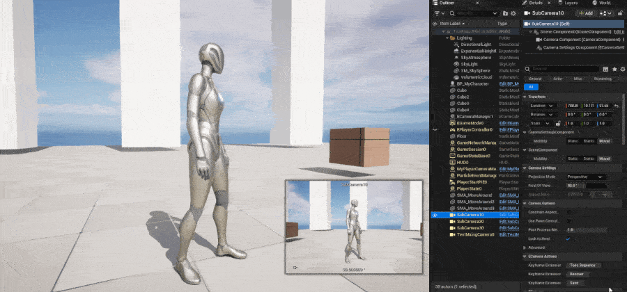
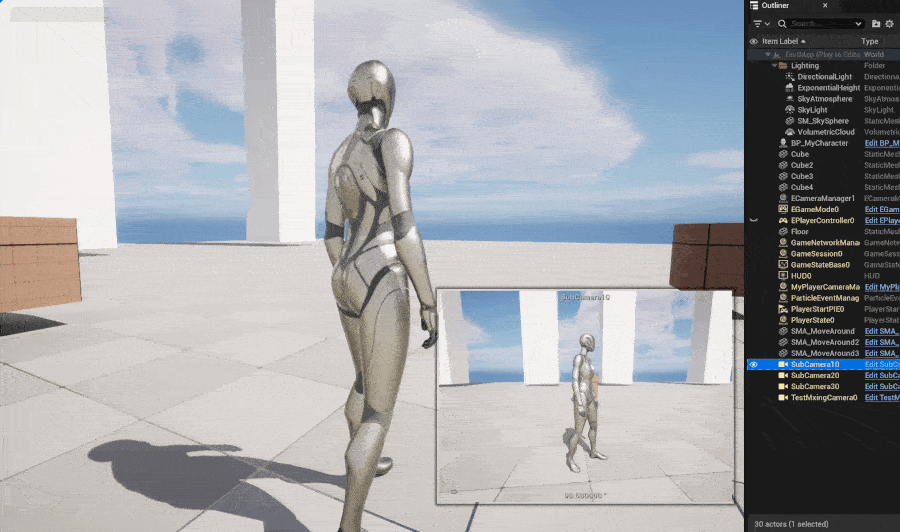
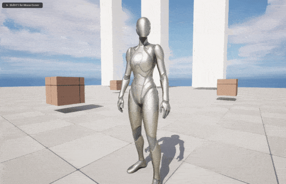
The following figure shows how M-lerp works to blend three sub-quaternions. Although you can observe that sometimes the camera rotates fast, it's generally continuous as sub-quaternions change without jump rotation. We can say that the averaged rotation is continuous but not continuous. I do not know if this statement is true. It's only my conjecture.

Theorem 4: Weight Continuity of M-lerp

In this subsection, we will show that the mapping of where is continuous on each . More formally, we have the following theorem:

Theorem 4: The mapping from a real value to the eigenvector of the largest eigenvalue of matrix is continuous.

We rewrite . We can then directly compute the derivative of with respect to :

which is constant over . This implies is continuous on . For any close enough to , and by Lemma 3.1, we know that:

where is the largest eigenvalue of and is the largest eigenvalue of where . It follows that:

where and are respectively the eigenvector of and , i.e., and .

Since is close enough to and by the fact that is continuous, there exists a matrix such that and . You can prove this by calculating the Frobenius norm of .

Then we can follow the same proof process of Theorem 3 to derive the conclusion.

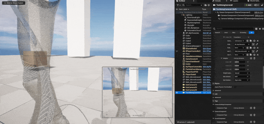
The following figure shows that unlike N-lerp, the averaged quaternion still maintains continuity as the weights change.

Method #3: Quaternion Flipping

The most common implementation of averaing rotations might be to maintain a running average and flip any incoming sub-rotation if the dot product between and is negative, i.e., it's on the opposite hemisphere to the running average.

FQuat RunningQuat = FQuat::Zero();

for (int i = 0; i < Quats.Num(); ++i)
{
    if (FQuat::Dot(RunningQuat, Quats[i]) >= 0)
    {
        RunningQuat = RunningQuat + Weights[i] * Quats[i];
    }
    else  // Flip
    {
        RunningQuat = RunningQuat - Weights[i] * Quats[i];
    }
}

RunningQuat.Normalize();

In this section, I will show that this method also introduces discontinuity in most cases, but it indeed grants continuity under certain conditions. If these conditions are satisfied in your application, you can safely use this approach to average rotations. We call this method F-lerp.

Theorem 5: Conditional Continuity of F-lerp

We first present a special case of F-lerp to give you an intuitive insight of how F-lerp ensures continuity.

Theorem 5: Given quaternions and their weights with , their F-lerp average rotation is continuous about at for some . All weights and other quaternions are fixed.

Proof is quite simple. assume the unnormalized quaternion in the -th iteration of F-lerp is , where can be or according to the F-lerp algorithm. When , the -th quaternion will be , so the product between and is . We can assume it's non-negative, so in the -th iteration of F-lerp the unnormalized quaternion is . Then for , , so the product will be negative, so the sign of will be flipped to . The unnormalized quaternion in the -th iteration of F-lerp will now become . This is the same as when . Proof completes.

Theorem 5 tells us that if all quaternions except the variable one are fixed, the average rotation derived from F-lerp is continuous about this rotation at , which is, as proved in Theorem 1, not continuous for N-lerp.

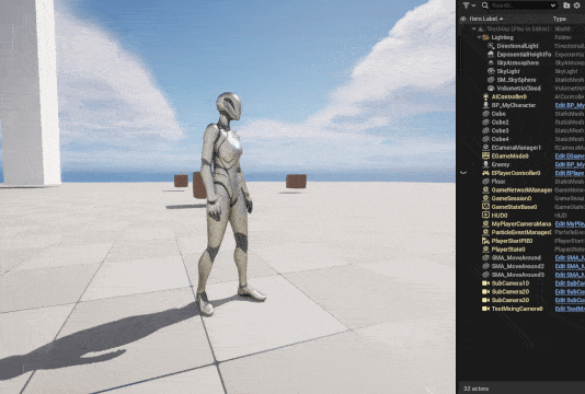
The following figure shows three rotations that are close enough are averaged without any discontinuity.

Theorem 5 rigorously assumes only one quaternion is variable. The following Corollary 5.1 presents a more general case where all quaternions are variable and the average quaternion is continuous about all of them, if satisfying certain conditions:

Corollary 5.1: Given quaternions and their weights with . All weights are fixed. Assume for some the quaternion lies in the neighborhood of and all other quaternions are not near . If (1) , and (2) or , then the F-lerp average rotation is continuous at where and all others are not.

Corollary 5.1 tells us that if one quaternion is crossing degree and the other quaternions are close enough (defined by two conditions: (1) their dot products are positive, and (2) their cosines have the same sign), the F-lerp result will not cause jump rotation when the quaternion crosses the boundary.

Let's proof it.

Let be the neighborhood of the rotation angle of with range and . Particularlly, , and for . Suppose . We also assume also rotation axes are fixed.

The -th iteration result of F-lerp can be written as (without normalization):

When , it's easy to know that according to the first condition.

When , we examine the value of respectively for and . It can be proved that is the same one, since we have and .

When , we can prove that . Taking , we can find that is continuous at that satistify the two conditions in the neighborhood.

You can similarly prove that if , at .

We have the following Corollary 5.2 to slightly relax the first condition of Corollary 5.1:

Corollary 5.2: Given quaternions and their weights with . All weights are fixed. Assume for some the quaternion lies in the neighborhood of and all other quaternions are not near . The F-lerp average rotation is continuous at where and all others are not, if the following conditions are satisfied:
(1) can be partitioned into two sets and and the two sets satisfy:
(1.1) ,
(1.2) .
(1.3) .
(2) or , and or .

The second condition says that the cosines of quaternions in the same set have the same sign, but the consines of quaternions from different sets are different.

Corollary 5.2 can be proved by progressively considering from , and . You should focus on the current sign of each quaternion added to .

Corollary 5.2 tells us that if all quaternions can be divided into two sets where (1) the intra-dot product is positive ( quaternions in the same set are close enough), (2) the inter-dot product is negative (quaternions from different sets are far away from each other), and (3) their rotation angles can also be separated by their cosine values, F-lerp then ensures continuity.

If you have a set of quaternions that are very close to each other, or two sets of quaternions that are separatable, you can use F-lerp to smoothly average quaternions.

Theorem 6: Discontinuity of F-lerp

In this section, I will show you that F-lerp also introduces discontinuities while eliminating some discontinuities brought by N-lerp. We have the following Theorem 6.

Theorem 6: Given quaternions and their associated weights with , the result of F-lerp has discontinuities if satisfying (1) , and (2) there exists a neighborhood of that makes the dot product change its sign, assuming and all are fixed and is variable. Here is the quaternion derived from the -th iteration of the F-lerp algorithm.

The intuition behind Theorem 6 is that as is continuous regarding all its elements, there should be some points at which the dot product between and changes its sign in the neighbourhood, i.e., from positive to negative or from negative to positive. This causes a significant difference between the two consecutive quaternions, giving rise to jump rotation. Note that by default, refers to the normalized result of the F-lerp algorithm though normalization is only applied at the final step in the original algorithm.

The key point is to find that makes . According to the definition of and , this gives us:

For example, when , this equation reduces to:

which implies that might be a discontinuity regardless of .

We can in fact estimate the difference between the quaternion where the dot product is positive and the quaternion where the dot product is negative.

Suppose the possible discontinuous quaternion is and in the positive neighborhood the dot product is positive, and in the negative neighborhood the dot product is negative. The rotation axis is fixed. Note that based on this assumption, cannot be as proven by Theorem 5. Besides, we assume in the neighborhood of the sign of dot product changes.

The positive result of F-lerp is (assume for ease of calculation):

Similarly, the negative result of F-lerp is:

It is obvious that taking limits for both and , the results are generally not equivalent:

and

The denominator seems a little crazy, but fortunately we can simplify it. Note that satisfy:

Then we have:

Next we expand the denominator of :

Therefore, we can rewrite and as:

The difference between and is determined by and . More importantly, we have , when is the quaternion that makes the dot product zero and there exists a neighborhood around that changes the sign of the dot product.

We can use a simple example to illustrate this. Suppose , a rotation around the -axis by , and , a rotation around the -axis by . This example satisfies the equation given at the beginning and there exists such that in the dot product changes its sign.

Then, we can easily calculate and as follows:

It is clear that means a rotation around the -axis by and is the identify rotation. The difference is .

The following figure illustrates that discontinuity does not appear at but at a point that makes the dot product zero. Jump rotation occurs.

The question, however, arises that any quaternion that makes the dot product zero is always a discontinuity? The answer is not always, but very likely to happen. If we assume , we can simplify the equation:

The root of it is , one of the two is within . If , it will get more complicated but there must also be discontinuities.

Remarks: F-lerp can be very helpful if you have a set of quaternions that are very close or two sets of quaternions that are separatable, but the risk is the result can be prone to discontinuities that are not , as shown in Theorem 6. If your quaternions are all around , F-lerp can be a very good choice -- it's smooth, fast, and will not trigger discontinuity.

Method #4: Smoothing the Discontinuity

C-lerp: Circular Mean as a Way of Average

Okay let's now forget about everything and think the very first question: why jump rotation happens? The answer is the illness of angle representation. The angle representation in game engine is or , both representing a full circle. In either case, we cannnot simply use the arithmetic mean to average angles because it's undirectional.

What about transforming the trivial angle representation into some other representation that is continuous regarding the input angle? Trigonometric functions, particularly cosine and sine functions, as we all know, serve this purpose quite well, since and .

Therefore, given a set of angles, we can first map them to the unit circle, i.e., converting from polar coordinates to Cartesian coordinates, compute the arithmetic mean of these points, and them map the averaged point back to the angle representation. This will be the final average angle we want.

More formally, assume are angles, we can use the following formula to calculate the average angle :

If each angle is weighted by , then the average angle would be:

This method is called C-lerp, short for circular interpolation, directly from the concept of Circular Mean.

We can write the pseudo code like:

float SumSinYaw = 0.f, SumCosYaw = 0.f;
float SumSinPitch = 0.f, SumCosPitch = 0.f;
float SumSinRoll = 0.f, SumCosRoll = 0.f;

for (int i = 0; i < Cameras.Num(); ++i)
{
   FRotator Q = Cameras[i]->GetActorRotation();
   
   SumSinYaw   += Weights[i] * FMath::DegSin(Q.Yaw);
   SumCosYaw   += Weights[i] * FMath::DegCos(Q.Yaw);
   SumSinPitch += Weights[i] * FMath::DegSin(Q.Pitch);
   SumCosPitch += Weights[i] * FMath::DegCos(Q.Pitch);
   SumSinRoll  += Weights[i] * FMath::DegSin(Q.Roll);
   SumCosRoll  += Weights[i] * FMath::DegCos(Q.Roll);
}

return FRotator(
   FMath::RadiansToDegrees(FMath::Atan2(SumSinPitch, SumCosPitch)),
   FMath::RadiansToDegrees(FMath::Atan2(SumSinYaw, SumCosYaw)), 
   FMath::RadiansToDegrees(FMath::Atan2(SumSinRoll, SumCosRoll))
);

The following figure gives two examples of how C-lerp works:

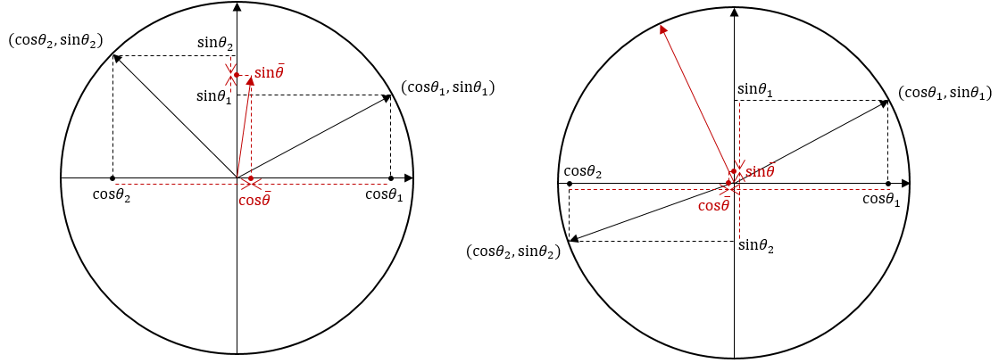
First, two angles are mapped to their Cartesian coordiantes and . Then the axis and axis values are independetly averaged as . Last, arctan is applied to convert the average point back to polar coordinates.

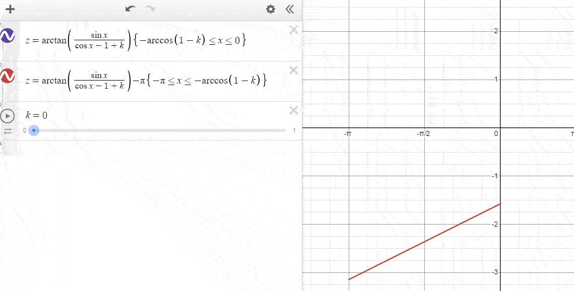
Looks perfect, right? However, unfortunately vanilla C-lerp does NOT ensure continuity. As a simple example, take and as a variable. According to C-lerp, the average angle would be:

It is obvious that is discontinuous at . When , whereas as . All the discontinuity is rooted in the discontinuity of the function, though and are continuous.

The following figure shows this discontinuity.

Albeit discontinuous at some points, C-lerp can replace L-lerp and F-lerp in most cases as there is less chance to trigger such discontinuity.

SC-lerp: Smoothed C-lerp

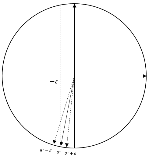
How to mitigate this sort of discontinuity caused by zero divided by zero? The most intuitive solution is to add a small positive number on the denominator side so that the denominator will always be positive, i.e.,

You can verify that is continuous about , as shown in the following figure.

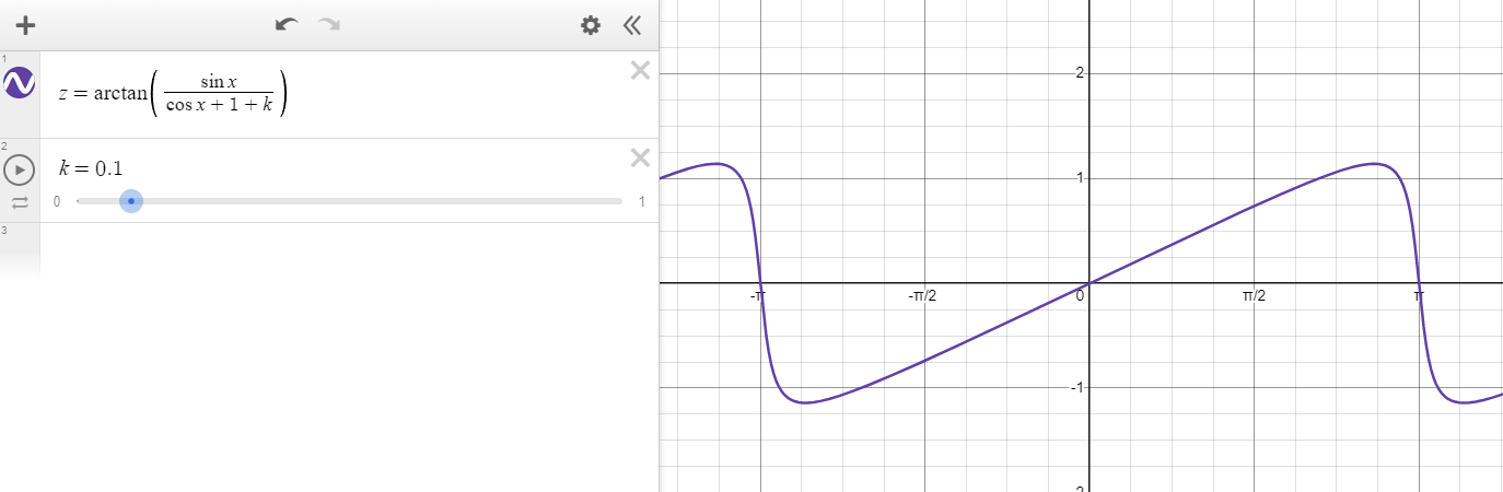
and here is the result:

Now the rotation becomes smooth at because the denominator will never get to zero and continuity is granted. But you may ask what about is not equal to 0 but instead. In this case, is calculated as follows:

Note that we cannot simply expand as since the denominator can become negative. Without loss of generality, let's assume and the root for equation is . Therefore, when , the denominator is positive, and the result can be expressed as:

but when , both the nominator and the denominator are negative, so the equation becomes:

Taking limits for both equations:

meaning that is continous on . You can similarly prove that it is also continous on , and hence is continuous on .

The following figure shows its continuity on :

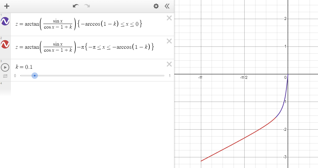
You can tweak the parameter to control how smooth the rotation will be at the root point. The larger is, the more smooth the result will be, but comes at the cost of curvature and accuracy.

Theorem 7: Continuity and Discontinuity of SC-lerp

In this secion, I present Theorem 7 to show when SC-lerp is continuous and discontinuous.

Theorem 7: Given angles where and the associated non-negative weights , the SC-lerped average angle is defined as , where . Let and . Then:
is continuous about each angle on domain if any of the following conditions is met:
(1) holds on .
(2) holds on .
(3) There exists such that and .
(4) There exists such that and and .
is discontinuous at if there exists such that and and .

Suppose is variable and all other angles plus all weights are fixed. The result of SC-lerp can be written as:

where is defined similar to the sign function:

Case 1
If holds on , is continuous on .

Case 2
If holds on , then we must discuss the sign of .

Case 2.1
If holds on , is continuous on .

Case 2.2
If holds on , is continuous on .

Case 2.3
There exists such that changes its sign in the neighborhood of . Assume when and when . Here is a small positive number. We then take limits for both sides:

is therefore continous on in this case.

Case 3
There exists such that and . This can be further divided into two cases.

Case 3.1
. In this case, changes its sign in the neighborhood of .

Assume when and when . Here is a small positive number. It's noteworthy that when is small enough, preserves its sign as , as shown in the following figure.

If we assume , then we can prove that . Based on our assumptions, we obtain that when , and when . Taking limits on both sides, we have:

Case 3.2
. In this case, preserves its sign in the neighborhood of .

If , we can obtain that by substituting into . Assume , then we can prove that , implying that it's continuous at . You can similarly prove the continuity at .

Case 4
There exists such that and . This can be further divided into three cases.

Case 4.1
. In this case, preserves its sign in the neighborhood while changes its sign.

If , we can obtain that and by substituting into and . It's obvious that is discontinuous at since and . The discontinuity also holds for .

Case 4.2
. In this case, changes its sign in the neighborhood but preserves its sign.

If , we have and . It's seen that is continuous at this point the limits for both sides are . This continuity also holds for .

Case 4.3
. In this case, both and change the signs. We can re-write them as and , so the result angle can be expressed as . We can compute the limit of the fraction:

is thus continous at .

To be short, is discontinuous at such that and and . In other cases, is continuous.

A decent value of depends on the circumstances you are in. can be positive or negative, and it can be large or small. Generally, if you set a relatively large , e.g., greater than or smaller than , that is discontinuous will be much less likely to happen, but a large value sacrifices average precision. You should be very careful of and tweak it for different situations.

The next three figures illustrate the results when is respectively , and . You will have a better understanding of how makes a difference to the final rotation.

Conclusion

In this article, I discussed several methods to average rotations: N-lerp (S-lerp), M-lerp, F-lerp, C-lerp and SC-lerp. I investigated the pros and cons of each method and proposed C-lerp and its improved version SC-lerp to average rotations in a simpler and more efficient way.

In summary, I suggest you:

• Use N-lerp if all sub-rotations are close enough and none of them cross from to (or from to );
• Use F-lerp if all sub-rotations are close enough or can be divided into two sets that are separatable;
• Use M-lerp if you want a smooth and accurate result;
• Use SC-lerp if you want a smooth and accurate result that is efficient to compute and the Euler angle interpolation does not make a big difference.

There might be mistakes in this article. Feel free to contact me if you find any / want to discuss with me / have further questions.

References

Averaging Quaternions
Quaternion Weighted Average
Perturbation Theory for Linear Operators
Circular Mean